Getting started with Machine Learning using Sklearn-python

Machine Learning and Artificial Intelligence are today's two hot topics that most attract the attention of researchers and the programmers.

With the enormous quantity and quality of available data today, there is an urge among many of us to find mysteries from several stones unturned. We know that many have already been turned, yet the newer scopes motivate us to find even the small pebbles, untrodden and unexplored.

Luckily, Machine Learning has this capability to analyze bigger and more complex data to find something that has been obscured from our mind.

Now, for the short introduction to the topic, what is Machine Learning? It is a method of data analysis that automates analytical model building. Using algorithms that iteratively learn from data, machine learning can find insights without being specially programmed for that purpose.

This post is dedicated to some of the basic algorithms that can help you get started with the topic using Python’s Sklearn.

First, you need to install this module using the pip install scikit-learn command on the terminal or command-prompt. Hopefully, sklearn will be installed successfully. You can also check by writing import sklearn on the Python interpreter.

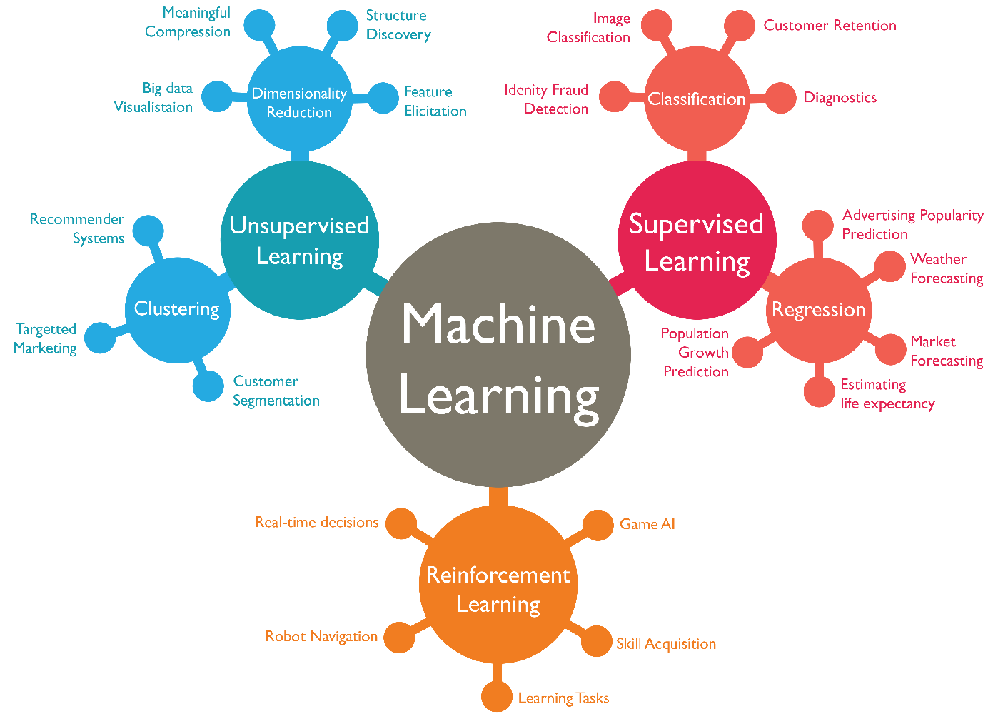
What are some important machine learning methods?

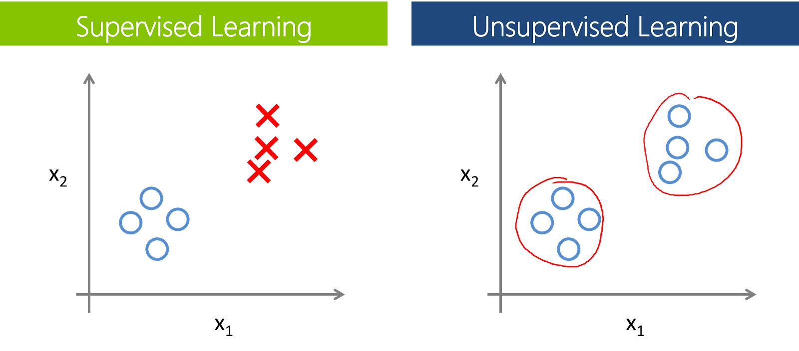
1. Supervised Learning algorithms are trained using pre-labeled data. Pre-labelled means we know the output of the training set that is given as the input to the model for learning purposes. Then we predict actual unlabelled data to get the answer to the desired question. For example, a part of the machine could have data points labelled either F (Failed) or R (Runs). The machine learning model receives this labelled set as the input with the labelled output and learns by comparing them to find the error between the predicted output and the actual output. Through methods like regression, classification, and prediction, supervised learning uses patterns to predict the values of the labels for another unlabelled data set.
2. Unsupervised learning is used against the data set that has no labels predefined. The model is not told the “right answer.” Instead, it must reach out to the conclusion to figure out what is being shown. Popular techniques include k-nearest neighbors, k-means clustering and self-organizing maps etc. These algorithms are used to recommend items, segment text topics and identify data outliers.

Besides these major methods, there are also the Semisupervised learning and Reinforcement learning methods. But, I am trying to keep this as short as possible so that you can get started very soon.

Here is the list of all important Supervised (labelled) learning algorithms and classification methods essential to learn the basics —

1. Naive Bayes
2. Decision Trees
3. Support Vector Machines (SVM)
4. Random Forests
5. AdaBoost

All of the above stated algorithms are very easy and similar to implement with sklearn. We need data in order to analyze it. The data is divided into two parts — training data and testing data.

The data points of the training dataset are very crucial in training the algorithmic model, no matter whatever it is and what type, whereas the testing dataset is the actual data we are interested in.

The desired model makes all of the necessary predictions using the testing dataset to reach out the answer to the question posed using actual dataset. Additionally, supervised learning also includes Features and Labels as the sub-parts of both training and testing datasets. Let us discuss them in brief in the next section.

Features and Labels

A feature or attribute is a quantity describing an instance. It has a domain defined as its attribute which is the key factor for deciding the values that it can take, whereas a label or target are the values and results assigned with each instance of the attribute as the output.

In a nutshell, feature is input while label is output.

Let us take an example of a person fond of listening to songs. Here, the features can be the intensity, tempo, genre, or gender of the singer, whereas whether the person likes or dislikes the song can be categorized as labels. Once you have trained your model, you will give it sets of new inputs as features and it will return the predicted labels (whether the person likes or dislikes the song) as the output.

Major Classification Algorithms

1. Naive Bayes algorithm  — Naive Bayes is one of the Classification technique based on applying Bayes’ theorem with strong (naive) assumptions between the features. Bayes’ theorem describes the probability of an event based on prior knowledge of the conditions that might be related to the event. Bayes' theorem is stated mathematically as the following equation: P(A∣B) = P(B∣A) . P(A) / P(B). To learn more about this mathematical term, follow the Naive Bayes’ link.

The Sklearn implementation of this classification algo is very easy.

>>> from sklearn import datasets
>>> iris = datasets.load_iris()
>>> from sklearn.naive_bayes import GaussianNB
>>> clf = GaussianNB()
>>> pred = clf.fit( iris.data, iris.target).predict(iris.data)

The first line imports the existing datasets module in Python. The second line loads the iris dataset into the iris variable . You can use any of the available datasets of your choice. The third line is just importing our Naive Bayes algo as Gaussian NaiveBayes.

Then, a classifier named clf is defined as an object for our model in the fourth line. The fit method in the fifth line fits the training dataset as features (data) and labels (target) into the Naive Bayes’ model.

The predict method predicts our actual testing dataset with regard to the fitted (training) data. This pred variable is our desired result of the testing dataset. It is a list containing the predictions corresponding to each and every data point in the dataset. For more details, please refer to the official documentation of Naive-Bayes’ Sklearn.

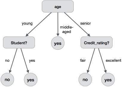
2. Decision Trees —  A Decision Tree is a decision support tool that uses a tree like graph or model of decisions and their possible consequences and reaches the final decision by following the entire path of the tree-like structure. A node of the tree is basically a condition. If the condition is true, the true part (sub-tree of a tree) is followed, else the false part. To know more about the Decision Trees algorithm, follow this link. The Sklearn implementation of this algorithm is below.

>>> from sklearn import tree
>>> X = [[0, 0], [1, 1]]
>>> Y = [0, 1]
>>> clf = tree.DecisionTreeClassifier()
>>> clf = clf.fit(X, Y)
>>> clf.predict([[2., 2.]])

The first line imports the tree class from sklearn module that contains DecisionTreeClassifier. The X and Y lists here denotes the features and target values of the training dataset. In the fourth line, we make object clf for the DecisionTreeClassifier class. After being fitted with the training data, the model can be used to predict the class of samples (training data). We can even obtain the predicted scores by comparing predicted data with target labels of the testing data. For more details, please refer to the official documentation of DecisionTreeClassifier Sklearn.

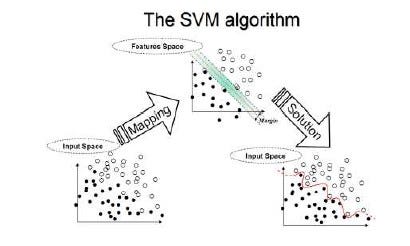
3. Support Vector Machines(SVM) — SVMs are supervised learning models with associated learning algorithms that analyze data used for classification. Given a set of training examples, each marked as belonging to one or the other of two groups, an SVM training algorithm builds a model that assigns new examples to one category or the other. An SVM model is the representation of the data as points in space, mapped so that examples of both the two categories are separated by a visible boundary or gap. To learn more about SVMs, follow this link. The Sklearn implementation of this algorithm is below.

>>> from sklearn import svm
>>> X = [[0, 0], [1, 1]]
>>> y = [0, 1]
>>> clf = svm.SVC()
>>> clf.fit(X, y)
>>> clf.predict([[2., 2.]])

This scikit-learn implementation is easy and following the general trend of using any classification model. Here, the first line, as usual, is importing the svm from sklearn standard library. The X and Y values correspond to the features and labels for the training dataset.

In the third line, we called Support Vector Classifier (SVC) class of the svm. There are several other available classes like LinearSVC, NuSVC, etc. Then, we fit this training set to help our model perform predictions on the testing dataset. In line 6, the model is used to predict the values for [[2., 2.]] dataset after being fitted. Then, we can also obtain the predicted scores for extra information by comparing predicted data with target labels of the testing data. For more details, please refer to the official documentation of SVM Sklearn.

4. Random Forests  — Random Decision Forests are an ensemble learning method for classification that operate by constructing the multitude of Decision Trees at training time and outputting the class that is the mode of classification. Random forests are a way of averaging multiple deep decision trees, trained on different parts of the same training set. Their predictive performance is better than that which could be made with a single decision tree algorithm. To learn more about Random Forests, follow this link.

The Sklearn implementation of this algorithm is below.

>>> from sklearn.ensemble import RandomForestClassifier
>>> X = [[0, 0], [1, 1]]
>>> Y = [0, 1]
>>> clf = RandomForestClassifier(n_estimators=10) 
>>> clf = clf.fit(X, Y)
>>> clf.predict(features_test)
>>> score = clf.score(features_test, labels_test)
>>> print score

Like the general trend in the line 1, we import RandomForestClassifier from python’s sklearn.ensemble module. Then, we make an object named clf as a classifier. In line 4, the parameter n_estimators refer to the number of decision trees used in the Random Forests model.

The fitting of the testing dataset makes the model ready for prediction. Then, we predict our actual dataset named features_test of the testing dataset. In line 7, the method score calculates the score (float value) of the actual features predicted with the true labels_test data.

Finally, we print the desired float value of the score of our model. The score here, is very useful in analyzing how accurate our model is. The higher value denotes more accuracy and success of implementation while lower values are less useful and usually results in the failure of our model. For more details, please refer to the official documentation of Random Forest Sklearn.

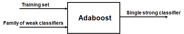
5. AdaBoost —AdaBoost, short for “Adaptive Boosting”, is a machine learning algorithm used in conjunction with many other types of algorithms to improve their performance. The output of the other learning algorithms (‘weak learners’) is combined into a weighted sum that represents the final output of the boosted classifier. AdaBoost is mostly sensitive to noisy data and outliers. AdaBoost is suitable with many learning algorithms. AdaBoost with Decision Trees as the weak learners, is often regarded as the best out-of-the-box classifier. To know more about AdaBoost, follow this link.

The Sklearn implementation of this algorithm is below.

>>> from sklearn.ensemble import AdaBoostClassifier 
>>> X = [[0, 0], [1, 1]]
>>> Y = [0, 1]
>>> clf = AdaBoostClassifier(n_estimators=50)
>>> clf = clf.fit(X, Y)
>>> clf.predict(features_test)
>>> score = clf.score(features_test, labels_test)
>>> print score.mean()

Until now, you should be very much familiar with the general way of using any learning model. Here also, we import AdaBoostClassifier from sklearn.ensemble module. In line 4, we make an object named elf (classifier) of AdaBoost type. It takes a parameter n_estimators meaning the maximum number of estimators at which boosting is terminated.

In case of a perfect fit, the learning procedure is stopped early. After that, the general procedure of fitting the training dataset occurs followed by the most important prediction part. The actual data is predicted using the model and scores are obtained after the result. score.mean() returns the mean accuracy on the given test data features_test and labels_test.

Finally, we print the desired float value of the score of our model. For more details, please refer to the official documentation of AdaBoost Sklearn.

Every learning algorithm tends to suit some problem types better than the others, and typically has many different parameters and configurations to be adjusted before achieving the optimal performance on a dataset.

Like I said earlier, machine learning based algorithms are rarely 100% accurate. We aren’t at the stage where Robocop driving his motorcycle at 100 mph can track criminals using low quality CCTV cameras… yet.

In fact, not a single algorithm is appropriate for solving every type of problem. We have to analyze the problem and dig out the most efficient and simple algorithm to answer the questions and analyze the obscured trends in the data.

Sometimes, the selection of suitable algorithms is not the only important task. We are required to tune our learning model as well by selecting the best parameter values taken by our learning classifier in order to obtain the maximum possible accuracy.

I hope this tutorial is helpful for you to get started with the basics. For any mistakes or further advancements, please let me know.