Deep Learning

Hi friends,

I am starting a series of blogs explaining the concept of Machine Learning and Deep Learning and will provide short notes from the following books, namely:

1. Deep Learning, by  Ian Goodfellow, Yoshua Bengio, and Aaron Courville

2. Machine Learning Probabilistic Perspective, by Kevin Murphy

3. The Elements of Statistical Learning, by  Trevor Hastie, Robert Tibshirani and Jerome Friedman

INTRODUCTION

Today, Artificial intelligence(AI) is a thriving field with many practical applications and active research topics. The true challenge to artificial intelligence is to solve problems that humans solve intuitively by observing things like spoken accents and faces in an image.

The solution to the above problem is to allow computers to learn from experience and understand the world in terms of a hierarchy of concepts, with each concept defined in terms of its relation to simpler concepts.

By gathering knowledge from experience, this approach avoids the need for human operators to formally specify all of the knowledge that the computer needs.

The hierarchy of concepts allows the computer to learn complicated concepts by building them out of simpler ones. If we draw a graph showing how these concepts are built on top of one another, the graph is deep, with many layers. For this reason, we call this approach AI deep learning.

Several artificial intelligence projects have sought to hard-code knowledge about the world in formal languages. A computer can reason about statements in these formal languages automatically, using logical inference rules.

This is known as the knowledge base approach to artificial intelligence. None of these projects have led to a major success. One of the most famous such projects is Cyc (Lenat and Guha, 1989).

It is not always possible to hard-core each feature in our machine. The ability to acquire their own knowledge is necessary and can be gained by extracting patterns from raw data.

This capability is known as machine learning. The performance of simple machine learning algorithms depends heavily on the representation of the data they are given. Each piece of information included in the representation of our desired problem is known as a feature (Fig 1).

Fig 1. Representation of image as possible feature

Importance of features is very crucial. For instance, human beings can easily perform arithmetic with Arabic numbers, but doing arithmetic with Roman numerals is much more time-consuming.

It is unsurprising that the choice of representation has an enormous effect on the performance of machine learning algorithms.

Fig 2. The importance of data representation: In the first plot, we have represented data in Cartesian coordinates and in second, data has been represented in Polar coordinates. In the second chart, the task becomes simple to solve with a vertical line. (photo courtesy: Deep Learning Book)

Now, to solve this problem, we can use machine learning – not only to discover mapping from representation to output, but also representation itself. This is called representation learning, i.e., learning representations of the data that make it easier to extract useful information when building classifiers or other predictors.

In the case of probabilistic models, a good representation is often one that captures the posterior distribution of the underlying explanatory factors for the observed input (we will revisit this topic later in greater detail). Talking about representational learning in terms of the autoencoder is a good example.

An autoencoder is the combination of an encoder function that converts the input data into a different representation and a decoder function that converts the new representation back into the original format.

Fig 3. Illustration of a deep learning model.

Of course, it can be very difficult to extract such high-level, abstract features from raw data. Many representations, such as a speaker’s accent, can be identified only using sophisticated, nearly human-level understanding of the data.

It is nearly as difficult to obtain a representation as it is to solve the original problem. Representation learning does not, at first glance, seem to help us.

Deep learning solves this central problem in representation learning by introducing representations that are expressed in terms of other, simpler representations.

Deep learning allows the computer to build complex concepts out of simpler concepts (Fig 3). There are two main ways of measuring the depth of a model (Fig 4).

1. Number of sequential instructions that must be executed to evaluate the architecture.
2. Depth of the graph describing how concepts are related to each other.

It is not always clear which of these two views  —  the depth of the computational graph, or the depth of the probabilistic modeling graph  —  is most relevant.

Because different people choose different sets of smallest elements from which to construct their graphs, there is no single correct value for the depth of an architecture, like there is no single correct value for the length of a computer program. Nor is there a consensus about how much depth a model requires to qualify as “deep.”

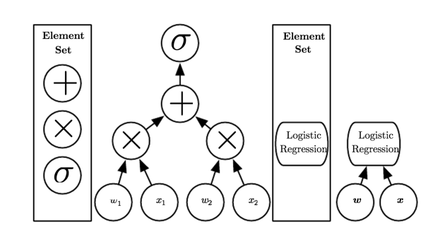
Fig 4. Illustration of computational graphs mapping an input to an output where each node performs an operation.

The division of various type of learning in Fig 5 will give you a great idea about the difference and similarity between them.

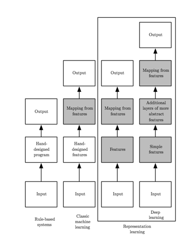
Fig 5. Flowcharts showing how the different parts of an AI system relate to each other within different AI disciplines. Shaded boxes indicate components that are able to learn from data. (photo courtesy: Deep Learning Book)

The earliest predecessors of modern deep learning were simple linear models. These models were designed to take a set of n input values x1, . . . , xn and associate them with an output y.

These models would learn a set of weights w1, . . . , wn and compute their output f(x, w) =x1*w1+···+xn*wn. This first wave of neural networks research was known as cybernetics.

In the 1950s, the perceptron (Rosenblatt, 1958, 1962) became the first model that could learn the weights defining the categories given examples of inputs from each category.

The adaptive linear element (ADALINE), which dates from about the same time, simply returned the value of f(x) itself to predict a real number (Widrow and Hoff, 1960), and could also learn to predict these numbers from data.

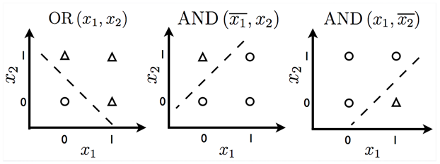
Fig 6. Functions which can be predicted by linear models.

Models based on the f(x, w) used by the perceptron and ADALINE are called linear models. Linear models have many limitations. Most famously, they cannot learn theXOR function, where f([0,1], w) = 1 and f([1,0], w) = 1 but f([1,1], w) = 0 and f([0,0], w) = 0 (Fig 7).

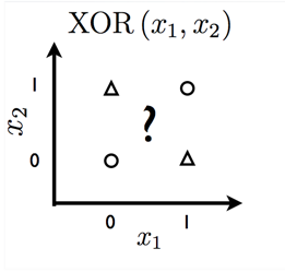
Fig 7. Cannot be solved by linear model.

This limitation of linear models has led to more sophisticated techniques. Today, Dataset Sizes
2. Increase Model Sizes
3. Increase Accuracy, Complexity, and Real-World Impact

Please provide your feedback so that I can improve in future articles.

Thanks all!

Articles in Sequence:

1. DEEP LEARNING
2. Deep Learning: Basic Mathematics for Deep Learning
3. Deep Learning: Feedforward Neural Network
4. Back Propagation

This post is originally published by the author here. This version has been edited for clarity and may appear different from the original post.