Deep Learning: Basic Mathematics for Deep Learning

Before getting started with neural networks and deep learning, lets discuss about the basic mathematics required to understand them. I will try to cover some important mathematics topic that would be required to understand further topics of deep learning.

LINEAR ALGEBRA

Linear algebra is a form of continuous rather than discrete mathematics, many computer scientists have little experience with it. A good understanding of linear algebra is essential for understanding and working with many machine learning algorithms, especially deep learning algorithms.

The study of linear algebra involves several types of mathematical objects they are as follows:

1. Scalars: A scalar is just a single number, in contrast to most of the other objects studied in linear algebra, which are usually arrays of multiple numbers. We write scalars in italics. We usually give scalars lower-case variable names.
2. Vectors: A vector is an array of numbers. The numbers are arranged in order. We can identify each individual number by its index in that ordering.Typically we give vectors lower case names written in bold typeface, such as x.
3. Matrices: A matrix is a 2-D array of numbers, so each element is identified by two indices instead of just one. We usually give matrices upper-case variable names with bold typeface, such as A.
4. Tensors: In some cases we will need an array with more than two axes.In the general case, an array of numbers arranged on a regular grid with a variable number of axes is known as a tensor. We denote a tensor named “A” with this typeface: A.

One important operation on matrices is the transpose. The transpose of a matrix is the mirror image of the matrix across a diagonal line, called the main diagonal , running down and to the right, starting from its upper left corner. We denote the transpose of a matrix A as A´ , and it is defined such that A´(i,j) = A(j,i).

In the context of deep learning, we also use some less conventional notation.We allow the addition of matrix and a vector, yielding another matrix: C = A + b , where C(i,j) = A(i,j) + b(j). In other words, the vector b is added to each row of the matrix. This shorthand eliminates the need to define a matrix with b copied into each row before doing the addition. This implicit copying of b to many locations is called broadcasting.

The transpose of a matrix product has a simple form: ( AB )´= B´A´. The matrix inverse of A is denoted as A^-1  , and it is defined as the matrix such that A^-1A = I (I is Identity matrix). However, A^−1 is primarily useful as a theoretical tool, and should not actually be used in practice for most software applications.Because A^−1 can be represented with only limited precision on a digital computer, algorithms that make use of the value of b can usually obtain more accurate estimates of x.

Some topics that need to be understand.

NORM

Sometimes we need to measure the size of a vector. In machine learning, we usually measure the size of vectors using a function called a norm. Given by:

Norms, including the L^p norm, are functions mapping vectors to non-negative values. On an intuitive level, the norm of a vector x measures the distance from the origin to the point x. More rigorously, a norm is any function f that satisfies the following properties:

• f ( x ) = 0 ⇒ x = 0
• f ( x + y ) ≤ f( x ) + f( y ) (the triangle inequality)
• ∀α ∈ R, f(α x ) = |α|f( x )

So we can say that The L² norm, with p= 2, is known as the Euclidean norm as it is simply Euclidean distance from origin.

EIGEN DECOMPOSITION

Many mathematical objects can be understood better by breaking them into constituent parts, or finding some properties of them that are universal, not caused by the way we choose to represent them. For example, integers can be decomposed into prime factors. The way we represent the number 12 will change depending on whether we write it in base ten or in binary, but it will always be true that 12 = 2×2×3. From this representation we can conclude useful properties, such as that 12 is not divisible by 5, or that any integer multiple of 12 will be divisible by 3.

In the same way we can also decompose matrices in ways that show us information about their functional properties. One of the most widely used kinds of matrix decomposition is called eigen-decomposition , in which we decompose a matrix into a set of eigenvectors and eigenvalues.

An eigenvector of a square matrix A is a non-zero vector v such that multiplication by A alters only the scale of v :

Av = λv

The scalar λ is known as the eigenvalue corresponding to this eigenvector. A visual representation of eigenvalue and eigenvector is show in Fig 1.

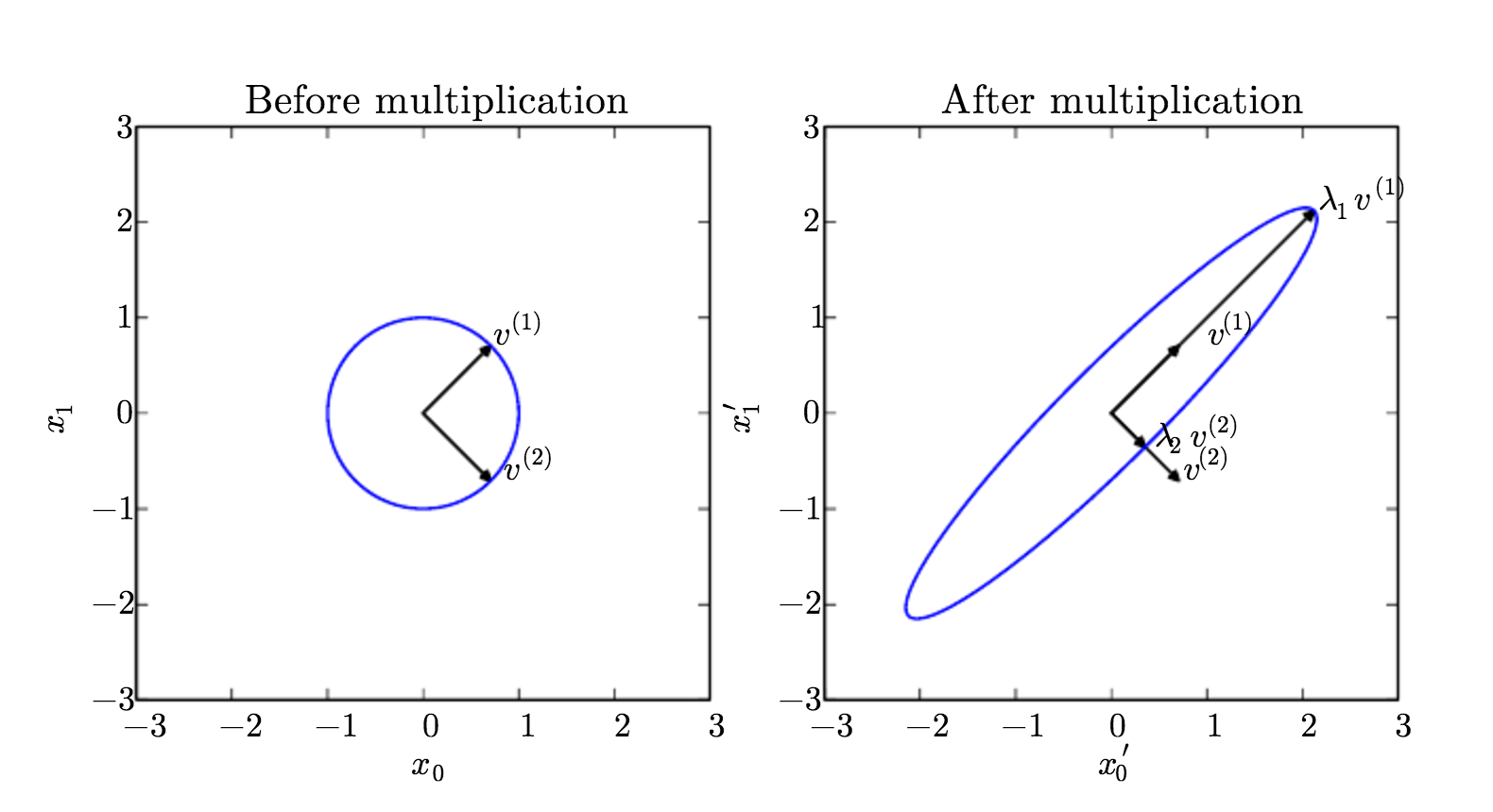
Fig 1. We have a matrix A with two orthonormal eigenvectors, v(1) with eigenvalue λ1 and v(2) with eigenvalue λ2. (Left) We plot the set of all unit vectors u ∈ R² as a unit circle. (Right) We plot the set of all points Au. By observing the way that A distorts the unit circle, we can see that it scales space in direction v(i) by λi. Image Courtesy: Deep Learning Book

The eigen decomposition of a matrix tells us many useful facts about the matrix.

1. The matrix is singular if and only if any of the eigenvalues are zero.
2. The eigen decomposition of a real symmetric matrix can also be used to optimize quadratic expressions of the form f( x ) = x ´ Ax subject to || x ||_2 = 1.

SINGULAR VALUE DECOMPOSITION

The singular value decomposition (SVD) provides another way to factorize a matrix, into singular vectors and singular values. The SVD allows us to discover some of the same kind of information as the eigen decomposition. However the SVD is more generally applicable. Every real matrix has a singular value decomposition, but the same is not true of the eigenvalue decomposition. For example, if a matrix is not square , the eigen decomposition is not defined, and we must use a singular value decomposition instead.

The singular value decomposition is similar, except this time we will write A as a product of three matrices:

A = U DV´.

Suppose that A is an m × n matrix. Then U is defined to be an m ×m matrix, D to be an m × n matrix, and V to be an n × n matrix. Each of these matrices is defined to have a special structure. The matrices U and V are both defined to be orthogonal matrices. The matrix D is defined to be a diagonal matrix. Note that D is not necessarily square. The elements along the diagonal of D are known as the singular values of the matrix A. The columns of U are known as the left-singular vectors. The columns of V are known as as the right-singular vectors.

The Moore-Penrose Pseudoinverse

Matrix inversion is not defined for matrices that are not square. Suppose we want to make a left-inverse B of a matrix A , so that we can solve a linear equation:

Ax = y
by left-multiplying each side to obtain x = By.

If A is taller than it is wide, then it is possible for this equation to have no solution. If A is wider than it is tall, then there could be multiple possible solutions.

The Moore-Penrose pseudoinverse allows us to make some headway in these cases. The pseudoinverse of A is defined as a matrix

(A+) = lim(α->0)( A´A + α I )ˆ−1 A ´.

Practical algorithms for computing the pseudoinverse are not based on this definition, but rather the formula

(A+)= V (D+) U´ ,

where U , D and V are the singular value decomposition of A, and the pseudoinverse D+ of a diagonal matrix D is obtained by taking the reciprocal of its non-zero elements then taking the transpose of the resulting matrix.

How it is significant ?

When A has more columns than rows, then solving a linear equation using the pseudoinverse provides one of the many possible solutions. Specifically, it provides the solution x = ( A+ ) y with minimal Euclidean norm || x ||² among all possible solutions.

When A has more rows than columns, it is possible for there to be no solution. In this case, using the pseudoinverse gives us the x for which Ax is as close as possible to y in terms of Euclidean norm || Ax − y ||².

Update:

The Hadamard product, s⊙t

suppose s and t are two vectors of the same dimension. Then we use s⊙t to denote the elementwise product of the two vectors. Thus the components of s⊙t are just ( s⊙t )j= s j t j. As an example,

Thanks

Please provide your feedbacks, so that I can improve in further articles.

Articles in Sequence:

1. DEEP LEARNING
2. Deep Learning: Basic Mathematics for Deep Learning
3. Deep Learning: Feedforward Neural Network
4. Back Propagation