Machine Learning with Python: Easy and robust method to fit nonlinear data

Easy and robust methodology for nonlinear data modeling using Python libraries, pipeline features, and regularization.

Nonlinear data modeling is a routine task in data science and analytics domain. It is extremely rare to find a natural process whose outcome varies linearly with the independent variables. Therefore, we need an easy and robust methodology to quickly fit a measured data set against a set of variables assuming that the measured data could be a complex nonlinear function. This should be a fairly common tool in the repertoire of a data scientist or machine learning engineer.

There are few pertinent questions to consider:

• How do I decide what order of polynomial to try to fit? Do I need to include cross-coupling terms for multi-variate regression? Is there an easy way to automate the process?
• How to ensure I don’t overfit to the data?
• Is my machine learning model robust against measurement noise?
• Is my model easily scalable to higher dimensions and/or to bigger data set?

How to decide the order of polynomial and related dilemma

“Can I plot the data and take a quick peek?”

That is OK only when one can visualize the data clearly (feature dimension is 1 or 2). It is lot tougher for feature dimensions 3 or higher. And it’s complete waste of time if there is cross-coupling within the features influencing the outcome. Let me show this by plots,

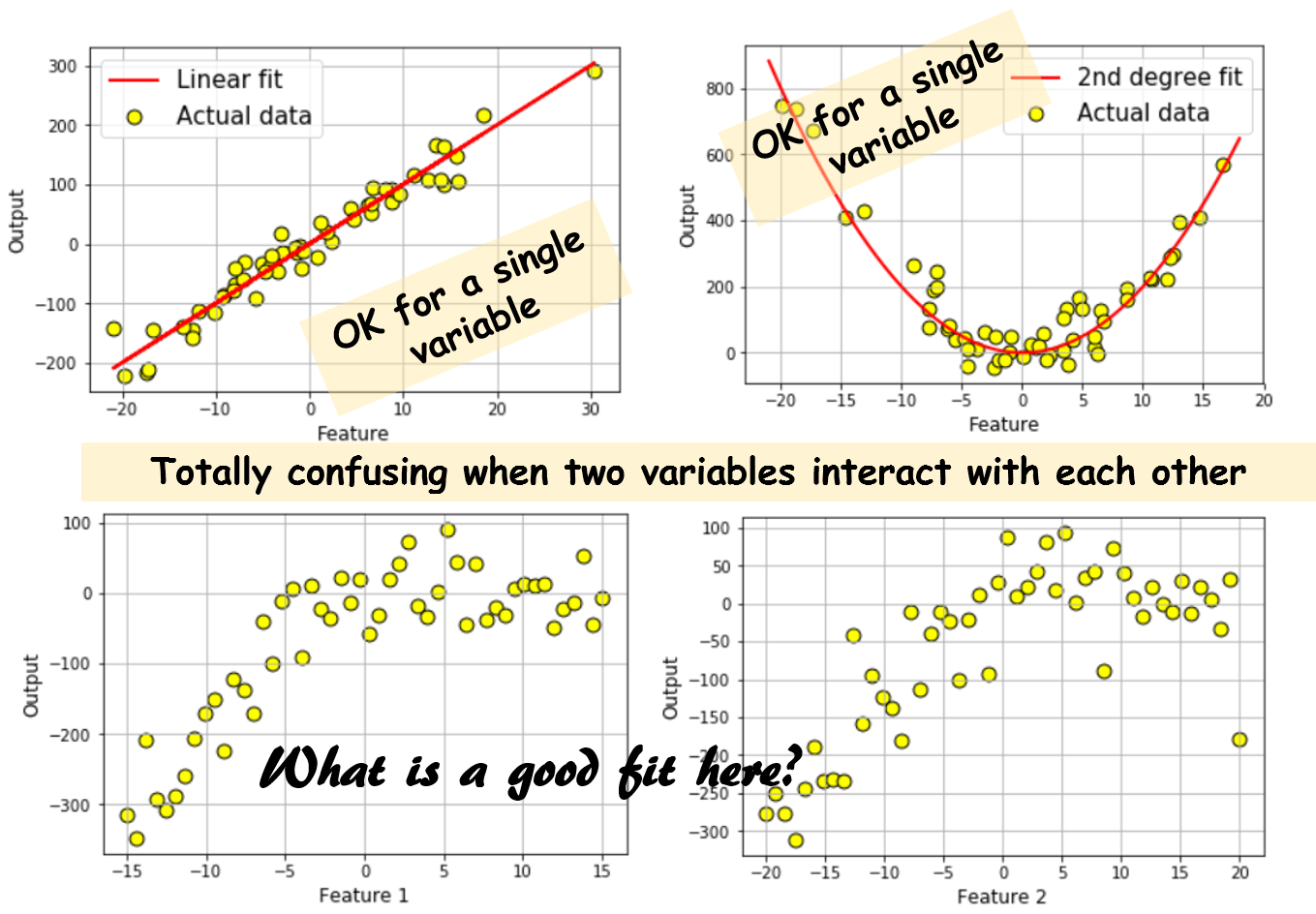
It is easy to see that plotting only takes you so far. For high-dimensional mutually-interacting data set, you can draw completely wrong conclusion if you try to look at the output vs. one input variable plot at a time. And, there is no easy way to visualize more than 2 variables at a time. So, we must resort to some kind of machine learning technique to fir a multi-dimensional dataset.

Actually, there are quite a few nice solutions out there.

Linear regression should be the first tool to look up and before you scream “…but these are highly nonlinear data sets…”, let us remember that the ‘LINEAR’ in linear regression model refers to the coefficients, and not to the degree of the features. Features (or independent variables) can be of any degree or even transcendental functions like exponential, logarithmic, sinusoidal. And, a surprisingly large body of natural phenomena can be modeled (approximately) using these transformations and linear model.

So, let’s say we get the following data set which has a single output and 3 features. We show the plots again, but, as expected, they don’t help much.

Therefore, we decide to learn a linear model with up to some high degree polynomial terms to fit a data set. Few questions immediately spring up:

— how to decide up to what polynomials are necessary

— when to stop if we start by incorporating 1st degree, 2nd degree, 3rd degree terms one by one?

— how to decide if any of the cross-coupled terms are important i.e. do we only need _X_1², _X_2³ or _X_1._X_2 and _X_1².X3 terms also?

— And finally, do we have to manually write equations/functions for all these polynomial transformations and add them to the data set?

Awesome Python Machine Learning Library to help

Fortunately, scikit-learn, the awesome machine learning library, offers ready-made classes/objects to answer all of the above questions in an easy and robust way.

Here is a simple video of the overview of linear regression using scikit-learn and here is a nice Medium article for your review . But we are going to cover much more than a simple linear fit in this article, so please read on. Entire boiler plate code for this article is available here on my GitHub repo.

We start by importing few relevant classes from scikit-learn,

# Import function to create training and test set splits
from sklearn.cross_validation import train_test_split

# Import function to automatically create polynomial features! 
from sklearn.preprocessing import PolynomialFeatures

# Import Linear Regression and a regularized regression function
from sklearn.linear_model import LinearRegression
from sklearn.linear_model import LassoCV

# Finally, import function to make a machine learning pipeline
from sklearn.pipeline import make_pipeline

Let us quickly define/recap the required concepts which we are going to use/implement next.

Train/Test split : This means creating two data sets from the single set we have. One of them (Training set) will be used to construct the model and another one (Test set) will be solely used to test the accuracy and robustness of the model. This is essential for any machine learning task, so that we don’t create model with all of our data and think the model is highly accurate (because it has ‘seen’ all the data and fitted nicely) but it performs badly when confronted with new (‘unseen’) data in the real world. Accuracy on the test set matters much more than the accuracy on training set. Here is a nice Medium article on this whole topic for your review. And below you can watch Google Car pioneer Sebastian Thrun talking about this concept.

Automatic polynomial feature generation : Scikit-learn offers a neat way to generate polynomial features from a set of linear features. All you have to do is to pass on the linear features in a list and specify the maximum degree up to which you want the polynomial degree terms to be generated. It also gives you choice to generate all the cross-coupling interaction terms or only the polynomial degrees of the main features. Here is an example Python code description.

Regularized regression : Importance of regularization cannot be overstated as it is a central concept in machine learning. In a linear regression setting, the basic idea is to penalize the model coefficients such that they don’t grow too big and overfit the data i.e. make the model extremely sensitive to noise in the data. There are two types of widely used regularization methods, of which we are using a method called LASSO. Here is a nice overview on both type of regularization methods.

Machine learning pipeline : A machine learning project is (almost) never a single modeling task. In its most common form, it consists of data generation/ingestion, data cleaning and transformation, model(s) fitting, cross-validation, model accuracy testing, and final deployment. Here is a Quora answer nicely summarizing the concept. Or, here is a related Medium article. Or, another nice article discussing the importance of pipeline practice. Scikit-learn offers a pipeline feature which can stack multiple models and data pre-processing classes together and turn your raw data into usable models.

If you have time, watch this long (1 hour +) video from PyData conference (Dallas, 2015) to see all of it in action.

How to build a robust model by putting it all together?

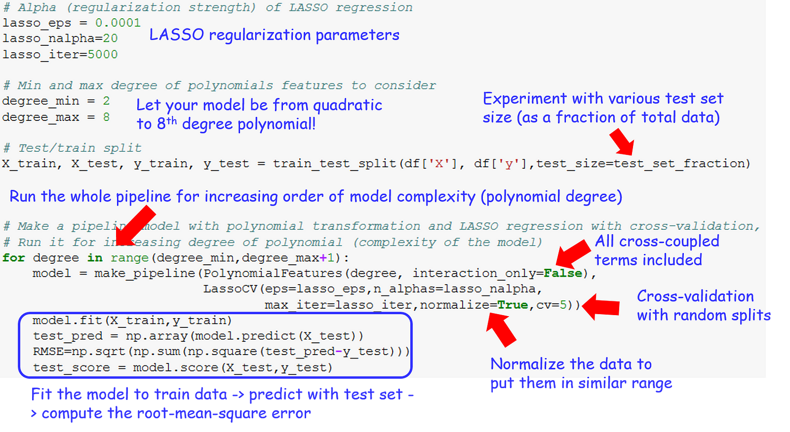
So, here is the boiler plate code snapshot. You must modify it to run properly for your data set.

# Alpha (regularization strength) of LASSO regression
lasso_eps = 0.0001
lasso_nalpha=20
lasso_iter=5000

# Min and max degree of polynomials features to consider
degree_min = 2
degree_max = 8

# Test/train split
X_train, X_test, y_train, y_test = 
train_test_split(df['X'], df['y'],test_size=test_set_fraction)

# Make a pipeline model with polynomial transformation and LASSO regression with cross-validation, run it for increasing degree of polynomial (complexity of the model)

for degree in range(degree_min,degree_max+1): 
  model = make_pipeline(PolynomialFeatures(degree, interaction_only=False),LassoCV(eps=lasso_eps,n_alphas=lasso_nalpha,max_iter=lasso_iter,normalize=True,cv=5)) 
    model.fit(X_train,y_train) 
    test_pred = np.array(model.predict(X_test))
    RMSE=np.sqrt(np.sum(np.square(test_pred-y_test))) 
    test_score = model.score(X_test,y_test)

But hey, code is for machines! For mere human, we need sticky notes. So, here is the annotated version of the same with notes and comments 

To distill it down further, here is the flow in more formal terms…

Let’s discuss the results!

For all the models, we also capture the test error, train error (root-mean-square), and the customary R² coefficient as the measure of model accuracy. Here is how they look like after we plot,

These plots are answering two of our earlier questions:

• We do need 4th or 5th degree polynomial to model this phenomena. Linear, quadratic, or even cubic models are not sufficiently complex for fitting the data.
• However, we should not need to go beyond 5th degree and over-complicate the model. Think this of a Occam’s Razor boundary for our model.

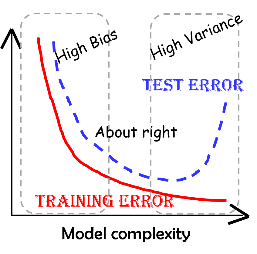
But, hey, where is the familiar bias/variance trade-off (aka underfit/overfit) shape in this curve? Why doesn’t the test error go up sharply for overly complex models?

The answer lies in the fact that using LASSO regression, we are essentially eliminating the higher-order terms in the more complex models. For more details, and some fantastic intuitive reasoning of why that happens, please read this article or watch the following video. This is, in fact, one of the key advantages of LASSO regression or L1-norm penalty, that it sets some of model coefficients to exactly zero instead of just shrinking them. Effectively, this does the ‘ automatic feature selection ’ for you i.e. let’s you automatically ignore the unimportant features even if you start with a highly complex model to fit the data.

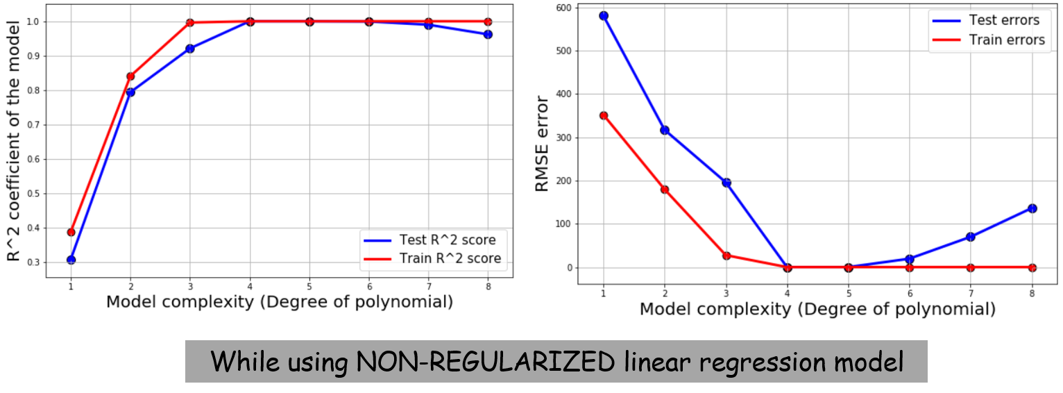
We can easily test this by NOT doing the regularization and using a simple linear regression model class from scikit-learn. Here is the result in that case. The familiar bias-variance shape is showing up for the model complexity vs. error plot.

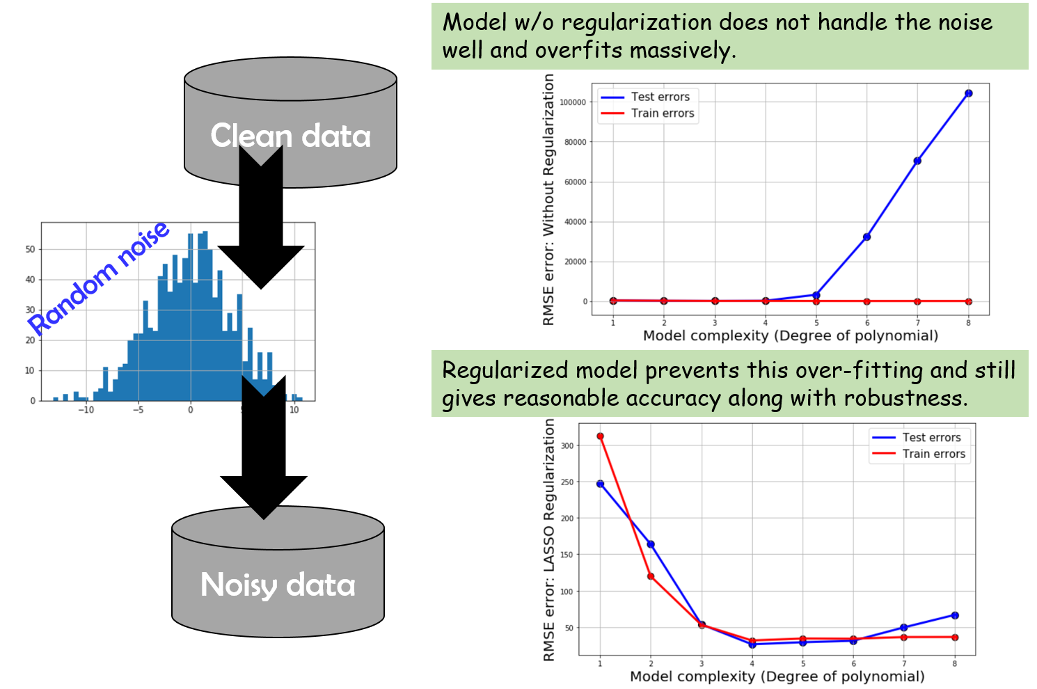
So, what happens with noisy data?

You can download my code and try changing the noise_magnitude parameter to see the impact of adding noise to the data set. Noise makes it hard for the model to be bias-free and it also pushes the model towards overfitting because the model tries to makes sense of the noisy data patterns and instead of discovering the real pattern, fits to noise. Basically, the simple linear regression model (w/o regularization) can fail miserable in this condition. The regularized model still fares well but the bias-variance trade-off starts showing up for even the regularized model performance. Here is the summary,

Epilogue

So, in short, we discussed a methodical way to fit multi-variate regression models to a data set with highly non-linear and mutually coupled terms, in the presence of noise. We saw how we can take advantage of Python machine learning library to generate polynomial features, normalize the data, fit the model, keep the coefficients from becoming too large thereby maintaining bias-variance trade-off, and plot the regression score to judge the accuracy and robustness of the model.

For more advanced types of model with non-polynomial features, you can check Kernel regression and Support Vector Regressor models from scikit-learn’s stable. Also, check this beautiful article about Gaussian kernel regression.

If you have any questions or ideas to share, please contact the author at tirthajyoti[AT]gmail[DOT]com. You can check author’s GitHub repositories for other fun code snippets in Python, R, or MATLAB and machine learning resources. Also, if you are, like me, passionate about machine learning/data science/semiconductors, please feel free to add me on LinkedIn or follow me on Twitter.