
gradientgmm: Fast Gaussian Mixtures in Scala
Gaussian Mixture Models(GMM) are arguably among the most popular clustering algorithms out there. They provide a concise probabilistic description of the data they are fitted to, and have been successfully applied in scientific fields that range from Astronomy to Genetics, among many others.
Evidence of their popularity is the ubiquity of their implementations: R, Python, Scala, Julia, C++, you name it.
A problem with such implementations, however, is that as the data set grow in size, they can become very slow; this is because typically they are implemented using the Expectation-Maximization, or EM, algorithm, which is a batch algorithm. This means that it has to go through all the data set at every iteration to take a step towards the solution. This seems rather inefficient: why don't we use instead some kind of stochastic gradient optimisation, which has showed its superior efficiency and speed time and time again in Deep Learning and other Machine Learning subdisciplines? well, it isn't so simple, but in this paper from 2017 such an algorithm was developed with the help of some cool maths, and implementing this result with a twist in Scala is exactly what I did for my MSc dissertation: using the mentioned paper as starting point, I created gradientgmm, a library with stochastic accelerated gradient descent algorithms for GMMs. This automatically allows the models to be tens or even hundreds of times faster than EM implementations for large datasets, and gives them other nice properties, like being able to handle streaming data. Let's try it out.
update: You can have a look at a quick explanation of the technical details in my personal site's post; I tried to keep it short though, so if you really want all the details have a look at the paper mentioned above by Hosseni and Sra.
Importing dependencies
I'm going to compare the model's results with the other GMM implementation in Scala: Spark MLlib's GaussianMixture. To import the Spark libraries and the GitHub projects, we just save the following build.sbt file in an empty folder:
scalaVersion := "2.11.8"
name := "gradientgmm-intro"
version := "1.0"

libraryDependencies  ++= Seq(
  "org.typelevel" %% "cats-core" % "1.0.1",
  "org.scalanlp" % "breeze_2.11" % "0.13.2",
  "org.scalanlp" % "breeze-natives_2.11" % "0.13.2",
  "org.scalanlp" % "breeze-viz_2.11" % "0.13.2",
   "org.apache.spark" % "spark-mllib_2.11" % "2.3.1",
  "org.apache.spark" % "spark-core_2.11" % "2.3.1"
)

lazy val githubDep1 = RootProject(uri("git://github.com/nestorSag/streaming-gmm#v1.5"))

lazy val githubDep2 = RootProject(uri("git://github.com/nestorSag/streaming-gmm-test#927ed81a01f60d29edb12275f9a431c0be05e75d"))

dependsOn(githubDep1)
dependsOn(githubDep2)
Once we do that, the remaining blocks of code can be ran in the sbt console from that folder. First, let's import the dependencies, and define some useful functions for comparing both implementations:
Setup
import com.github.gmmtest.CSeparatedDataGenerator

import com.github.gradientgmm.components._
import com.github.gradientgmm._
import com.github.gradientgmm.optim._

import org.apache.spark.mllib.stat.distribution.{MultivariateGaussian => SMG}
import org.apache.spark.mllib.clustering.{GaussianMixture, GaussianMixtureModel}
import org.apache.spark.mllib.linalg.{Matrix => SM, Vector => SV, Vectors => SVS, Matrices => SMS}

import org.apache.spark.SparkContext
import org.apache.spark.SparkConf

import breeze.linalg.{DenseVector => BDV, DenseMatrix => BDM}

//initialise Spark context
val conf = new SparkConf().setAppName("gradientgmm-test").setMaster("local[4]")
val sc = new SparkContext(conf)

//code block timer
//method from https://stackoverflow.com/a/9160068/5016440
def time[R](block: => R): R = {
   val t0 = System.nanoTime()
   val result = block    // call-by-name
   val t1 = System.nanoTime()
   println("Elapsed time: " + (t1 - t0) + "ns")
   result
}

def evaluateLogLikelihood(
 pt: BDV[Double],
 dists: Array[UpdatableGaussianComponent],
 weights: Array[Double]): Double = {
   val p = weights.zip(dists).map {
     	case (weight, dist) =>  weight * dist.pdf(pt)
   }
   for(i <- 0 to p.length-1){
     p(i) = math.min(math.max(p(i),Double.MinPositiveValue),Double.MaxValue/p.length)
   }
   val pSum = p.sum
   math.log(pSum)
}
Generating the data
I'm going to use synthetic data generated from a random, true GMM. The classes that do this are in the gradient-gmm repository we imported above. Let's initialise the generator and get a training data set.
val dim = 30 //data dimensionality
val k = 4 //number of clusters in the data
val c = 0.2 //clusters relative separation
val seed = 1 //random seed
val n = 200000 //number of data points

val generator = new CSeparatedDataGenerator(dim,k,c,seed)

val data = generator.draw(n)
The c parameter controls how separated the different Gaussian components are; the lower the separation the more mixing between them and the harder it is for an algorithm to fit the data and find the true parameters. If you are wondering, the formal deffinition is that a GMM is C-separated if and only if

Above, 3-component GMM with with c=1
Above, 3-component GMM withc=2

The Optimizer Object
If you've ever used stochastic gradient descent before, you will know that, unlike with the EM algorithm, you have a few parameters to tune. This is still true for GMMs, so let's set the optimisation algorithm we will use, which will be Nesterov accelerated gradient descent:
//set up the optimiser
val optim = new NesterovGradientAscent()
          .setLearningRate(0.9)
          .halveStepSizeEvery(30)
          .setMinLearningRate(1e-4) //step size won't get below this
          .setGamma(0.5) //Nesterov momentum parameter
Empirically, what worked best for GMMs was setting a high initial learning rate that shrinks as the optimisation goes by, until a minimum allowed step size; that is what the first three setters do.
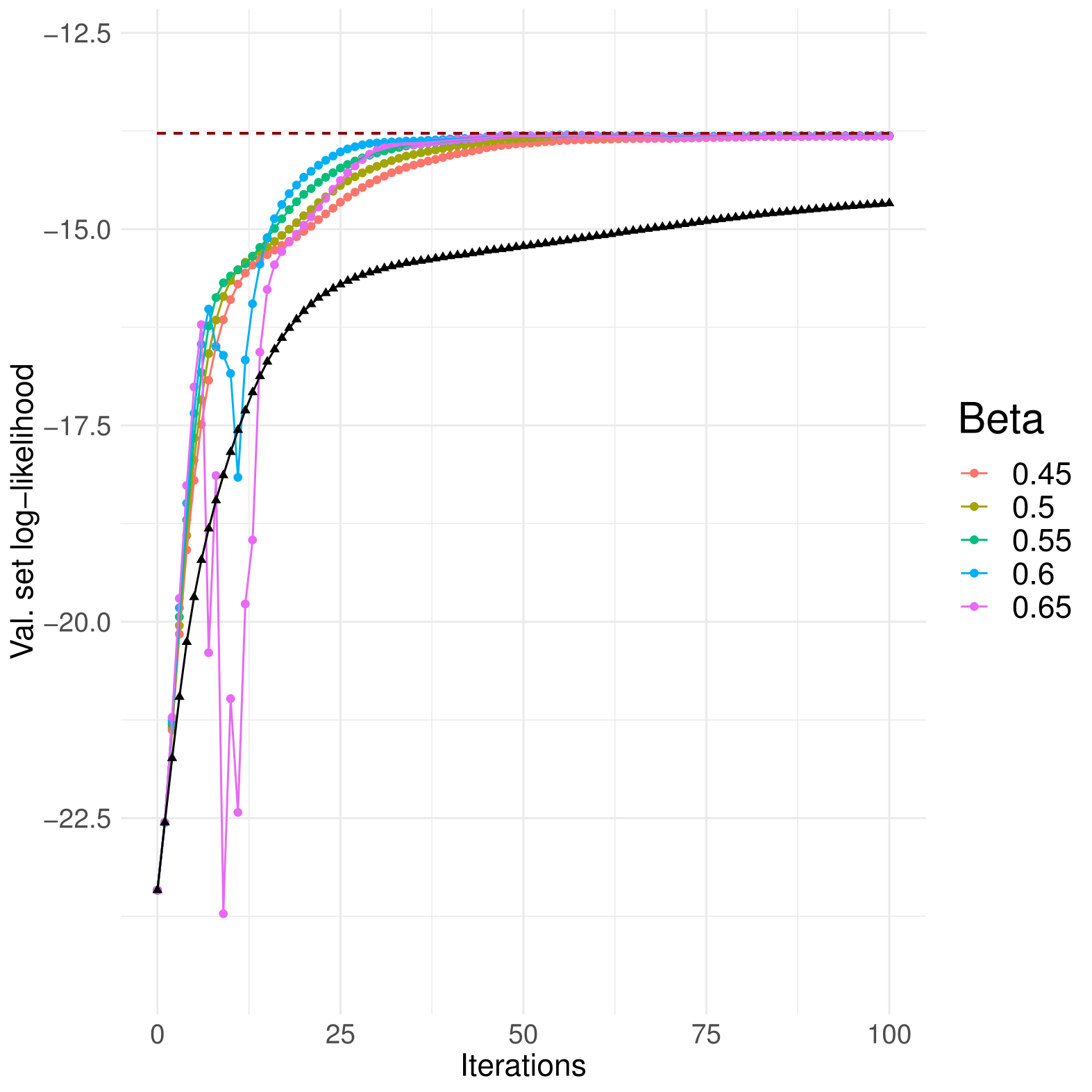
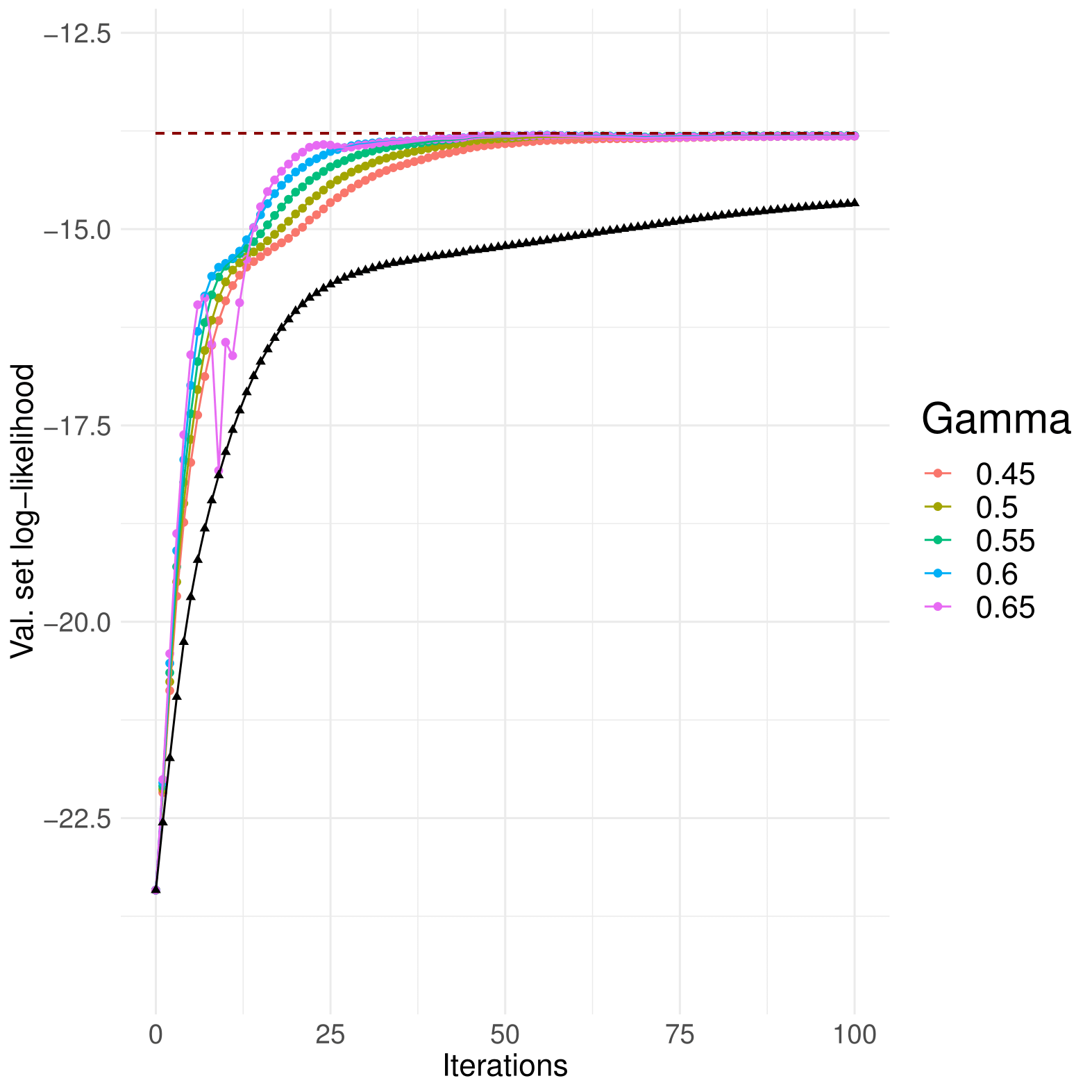
There are 3 optimisiation methods available : GradientAscent, MomentumGradientAscent and NesterovGradientAscent. It is emphatically recommended that you use one of the last two, since accelerated ascent worked much better than standard gradient ascent. Momentum parameters near 0.5 work well for both.
Above, Momentum ascent compared to standard gradient ascent, in black
Above, Nesterov ascent compared to standard gradient ascent, in black
Training The Model
To train the models we run the following blocks of code
//initial random means, uniform weights and identity covariances
val weights0 = (1 to k).map{case j => 1.0/k}.toArray
  var means0 = (1 to k).map{case j => (BDV.rand(dim) - 0.5) * 2.0}.toArray
  var vars0 = (1 to k).map{case j=> BDM.eye[Double](dim)}.toArray
  val gaussians0 = (1 to k).map{case j=> UpdatableGaussianComponent(means0(j-1),vars0(j-1))}.toArray

//initialise model
val model = GradientGaussianMixture(weights0,means0,vars0,optim)

//train the model
time { model
  .setMaxIter(200)
  .setBatchSize(1000)
  .step(data)
}
The first block creates the initial parameters the model is going to have: random centers, identity covariance matrices and uniform weights. The model can also be initialised with the results of a Spark's KMeans run using a small sample. This is done with the init() method and you can find more in the documentation. For now let's use random initialisation. After initialising the model in the second block, we fit it and time it with the last one.
Training the Spark Model
We now train the Spark's model, which uses the EM algorithm. To make things fair, we initialise it with the same initial guesses than our model.
val sparkGmm = new GaussianMixtureModel(
  weights0,
  means0.zip(vars0).map{case (m,v) => new SMG(SVS.dense(m.toArray),SMS.dense(dim,dim,v.toArray))})

val sparkGm = new GaussianMixture()
.setK(k)
.setInitialModel(sparkGmm)

val parallelData = sc.parallelize(data).map{case x => SVS.dense(x.toArray)}

val sparkModel = time {
   sparkGm.run(parallelData)
}
Comparing Results
By this point we have the processing time for both models in the screen, and we now proceed to calculate a the average log-likelihood for each model in a sample to evaluate their quality. All the results are shown below.
val valSample = generator.draw(10000)
//initial loglikelihood
val initialLL = valSample.map{
     case x => evaluateLogLikelihood(x, gaussians0, weights0)}.sum/valSample.length

val sparkLL = valSample.map{
    case x => evaluateLogLikelihood(x, sparkModel.gaussians.map(UpdatableGaussianComponent(_)) , sparkModel.weights)}.sum/valSample.length

val gradientLL = valSample.map{
    case x => evaluateLogLikelihood(x, model.getGaussians, model.getWeights)}.sum/valSample.length

//true gaussian parameters
val trueGaussians = generator.gaussians.map{
    case g => UpdatableGaussianComponent(
      g.mean,
      g.covariance)
}

val trueLL = valSample.map{
    case x => evaluateLogLikelihood(x, trueGaussians,          generator.weights.toArray)}.sum/valSample.length

println(s"trueLL: ${trueLL}, gradientLL: ${gradientLL}, sparkLL: ${sparkLL}, initialLL: ${initialLL}")
Running it all in my machine, which has a Intel® Core™ i7-4500U CPU @ 1.80GHz × 4 processor and 16GB of RAM, I got the following results:
| Model | LL value |
|---|---|
| True Model | -18.59 |
GaussianMixture |
-18.62 |
GradientGaussianMixture |
-18.77 |
| Initial Model | -47.10 |
| Algorithm | Time (s) |
|---|---|
GradientGaussianMixture |
6.52 |
GaussianMixture |
91.17 |
We got virtually the same results than Spark's model, but 14 times faster! that summarises the whole purpose of this model. It is worth noting that as the dataset size increases the difference in processing times becomes even more dramatic, because the processing time is independent from the dataset size for mini-batch algorithms, but not for batch algorithms: Using datasets with 4 million vectors, I saw speedups of 100x for some data configurations, even when Spark was using two 8-core machines.
Also, we have to note that the price we pay for the huge speedup is a higher error in parameter estimation, because at each iteration we use a small sample to estimate the true descent direction, and this introduces additional variance. Still, as we've seen above, this difference is quite small.
Distributed and Streaming data
GradientGaussianMixture can also work with Spark data in a distributed manner, without additional effort from the developer; we just need to pass the RDD full of Spark's DenseVectors.
Unfortunately, working with distributed Spark data negates the beneffits from mini-batch gradient descent, because without HPC networking, communication and synchronisation times take a big toll on speed. Since the maximum performance is achieved with sequential mini-batch processing, probably the best option for data that doesn't fit in memory would be creating two processes in the same machine, where one fetches a new data batch from the database while the other runs the optimisation with the current batch.
That being said, the model is perfect for streaming data, because it allows online learning, and it even has a forgetfullness rate built into it. The following lemma formalises this statement:
Lemma Let . For a step size of , the contribution of former Gaussian parameter values to the current state of the model decays at a rate of per iteration.
This is perfect for tuning the learning rate parameter using application-specific knowledge about the data stream. If you are curious, you can find the proof of this statement here, in the appendix.
The model is also able to process Spark's DStreams; the following are results I got running it in a small Databricks cluster with 8-core, 15GB RAM, 2.3GHz instances
| Machines | Samples | Dim | TIme(s) |
|---|---|---|---|
| 4 | 220,000 | 30 | 0.97 |
| 3 | 180,000 | 30 | 0.97 |
| 2 | 165,000 | 30 | 0.99 |
| 1 | 135,000 | 30 | 0.91 |
| 4 | 140,000 | 50 | 0.99 |
| 3 | 123,000 | 50 | 0.98 |
| 2 | 110,000 | 50 | 0.98 |
| 1 | 95,000 | 50 | 0.93 |
Final Remarks
gradientgmm is an excellent choice for users that need to fit data with a few hundred thousands to many millions of observations quickly. The speedup allows for much more experimentation with model parameters. It is also ideal as a clustering model for data streams.
The library also implements regularisation by logarithmic barrier to avoid covariance singularity issues and to make the model robust to anomalous data. If interested, you can find the full documentation here. and the project repository here