My last tutorial went over Logistic Regression using Python. One of the things learned was that you can speed up the fitting of a machine learning algorithm by changing the optimization algorithm. A more common way of speeding up a machine learning algorithm is by using Principal Component Analysis (PCA). If your learning algorithm is too slow because the input dimension is too high, then using PCA to speed it up can be a reasonable choice. This is probably the most common application of PCA. Another common application of PCA is for data visualization.

To understand the value of using PCA for data visualization, the first part of this tutorial post goes over a basic visualization of the IRIS dataset after applying PCA. The second part uses PCA to speed up a machine learning algorithm (logistic regression) on the MNIST dataset.

With that, let’s get started! If you get lost, I recommend opening the video below in a separate tab.

PCA using Python Video

The code used in this tutorial is available below

PCA for Data Visualization

PCA to Speed-up Machine Learning Algorithms

Getting Started (Prerequisites)

If you already have anaconda installed, skip to the next section. I recommend having anaconda installed (either Python 2 or 3 works well for this tutorial) so you won’t have any issue importing libraries.

You can either download anaconda from the official site and install on your own or you can follow these anaconda installation tutorials below to set up anaconda on your operating system.

Install Anaconda on Windows: Link

Install Anaconda on Mac: Link

Install Anaconda on Ubuntu (Linux): Link

PCA for Data Visualization

For a lot of machine learning applications it helps to be able to visualize your data. Visualizing 2 or 3 dimensional data is not that challenging. However, even the Iris dataset used in this part of the tutorial is 4 dimensional. You can use PCA to reduce that 4 dimensional data into 2 or 3 dimensions so that you can plot and hopefully understand the data better.

Load Iris Dataset

The Iris dataset is one of datasets scikit-learn comes with that do not require the downloading of any file from some external website. The code below will load the iris dataset.

import pandas as pd

url = "https://archive.ics.uci.edu/ml/machine-learning-databases/iris/iris.data"

# load dataset into Pandas DataFrame
df = pd.read_csv(url, names=['sepal length','sepal width','petal length','petal width','target'])

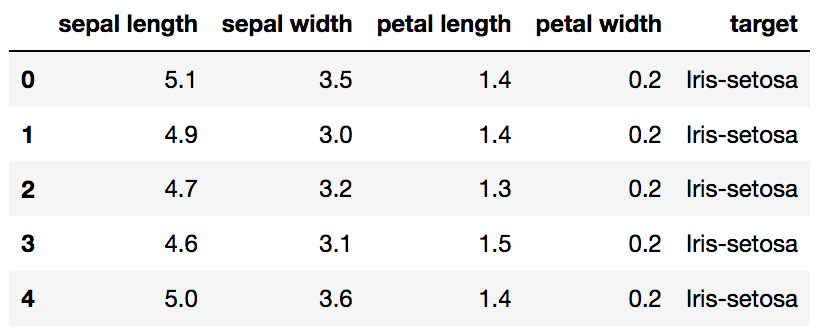
Original Pandas df (features + target)

Standardize the Data

PCA is effected by scale so you need to scale the features in your data before applying PCA. Use StandardScaler to help you standardize the dataset’s features onto unit scale (mean = 0 and variance = 1) which is a requirement for the optimal performance of many machine learning algorithms. If you want to see the negative effect not scaling your data can have, scikit-learn has a section on the effects of not standardizing your data.

from sklearn.preprocessing import StandardScaler
features = ['sepal length', 'sepal width', 'petal length', 'petal width']

# Separating out the features
x = df.loc[:, features].values

# Separating out the target
y = df.loc[:,['target']].values

# Standardizing the features
x = StandardScaler().fit_transform(x)

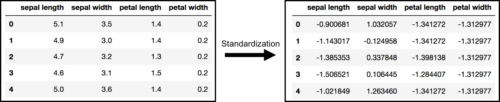
The array x (visualized by a pandas dataframe) before and after standardization

PCA Projection to 2D

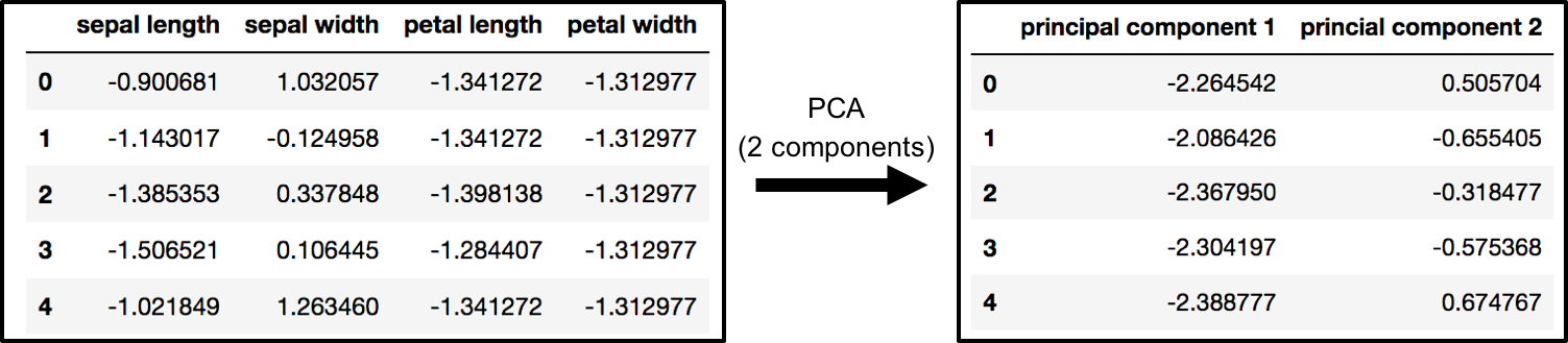
The original data has 4 columns (sepal length, sepal width, petal length, and petal width). In this section, the code projects the original data which is 4 dimensional into 2 dimensions. I should note that after dimensionality reduction, there usually isn’t a particular meaning assigned to each principal component. The new components are just the two main dimensions of variation.

from sklearn.decomposition import PCA

pca = PCA(n_components=2)

principalComponents = pca.fit_transform(x)

principalDf = pd.DataFrame(data = principalComponents , columns = ['principal component 1', 'principal component 2'])

PCA and Keeping the Top 2 Principal Components

finalDf = pd.concat([principalDf, df[['target']]], axis = 1)

Concatenating DataFrame along axis = 1. finalDf is the final DataFrame before plotting the data.

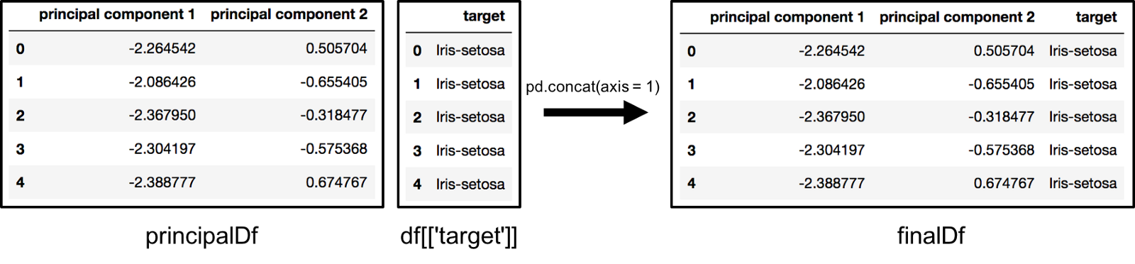
Concatenating dataframes along columns to make finalDf before graphing

Visualize 2D Projection

This section is just plotting 2 dimensional data. Notice on the graph below that the classes seem well separated from each other.

fig = plt.figure(figsize = (8,8))
ax = fig.add_subplot(1,1,1) 
ax.set_xlabel('Principal Component 1', fontsize = 15)
ax.set_ylabel('Principal Component 2', fontsize = 15)
ax.set_title('2 component PCA', fontsize = 20)
targets = ['Iris-setosa', 'Iris-versicolor', 'Iris-virginica']
colors = ['r', 'g', 'b']
for target, color in zip(targets,colors):
    indicesToKeep = finalDf['target'] == target
    ax.scatter(finalDf.loc[indicesToKeep, 'principal component 1']
               , finalDf.loc[indicesToKeep, 'principal component 2']
               , c = color
               , s = 50)
ax.legend(targets)
ax.grid()

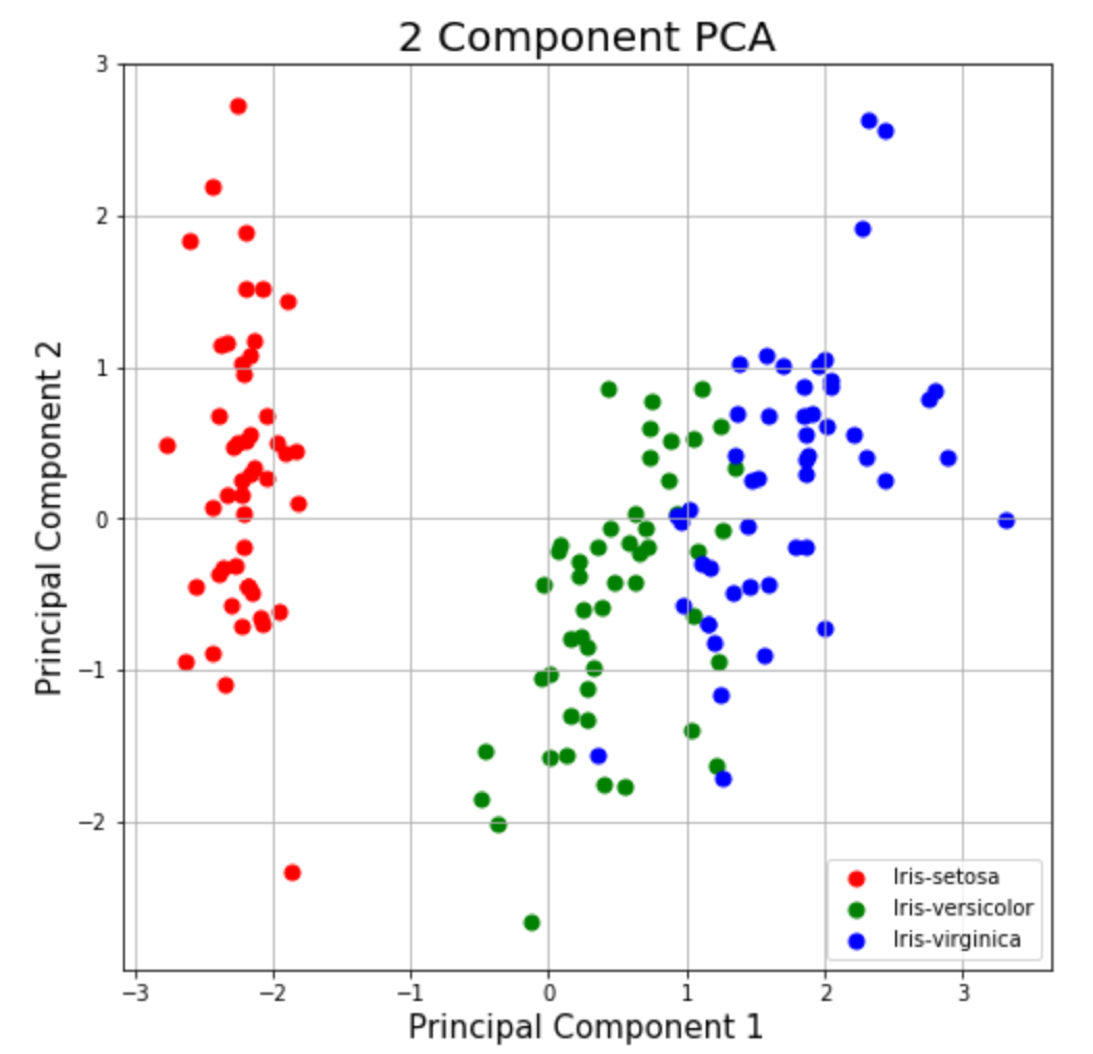
2 Component PCA Graph

Explained Variance

The explained variance tells you how much information (variance) can be attributed to each of the principal components. This is important as while you can convert 4 dimensional space to 2 dimensional space, you lose some of the variance (information) when you do this. By using the attribute explained_variance_ratio_ , you can see that the first principal component contains 72.77% of the variance and the second principal component contains 23.03% of the variance. Together, the two components contain 95.80% of the information.

pca.explained_variance_ratio_

PCA to Speed-up Machine Learning Algorithms

One of the most important applications of PCA is for speeding up machine learning algorithms. Using the IRIS dataset would be impractical here as the dataset only has 150 rows and only 4 feature columns. The MNIST database of handwritten digits is more suitable as it has 784 feature columns (784 dimensions), a training set of 60,000 examples, and a test set of 10,000 examples.

Download and Load the Data

You can also add a data_home parameter to fetch_mldata to change where you download the data.

from sklearn.datasets import fetch_mldata

mnist = fetch_mldata('MNIST original')

The images that you downloaded are contained in mnist.data and has a shape of (70000, 784) meaning there are 70,000 images with 784 dimensions (784 features).

The labels (the integers 0–9) are contained in mnist.target. The features are 784 dimensional (28 x 28 images) and the labels are simply numbers from 0–9.

Split Data into Training and Test Sets

Typically the train test split is 80% training and 20% test. In this case, I chose 6/7th of the data to be training and 1/7th of the data to be in the test set.

from sklearn.model_selection import train_test_split

# test_size: what proportion of original data is used for test set
train_img, test_img, train_lbl, test_lbl = train_test_split( mnist.data, mnist.target, test_size=1/7.0, random_state=0)

Standardize the Data

The text in this paragraph is almost an exact copy of what was written earlier. PCA is effected by scale so you need to scale the features in the data before applying PCA. You can transform the data onto unit scale (mean = 0 and variance = 1) which is a requirement for the optimal performance of many machine learning algorithms. StandardScaler helps standardize the dataset’s features. Note you fit on the training set and transform on the training and test set. If you want to see the negative effect not scaling your data can have, scikit-learn has a section on the effects of not standardizing your data.

from sklearn.preprocessing import StandardScaler
scaler = StandardScaler()

# Fit on training set only.
scaler.fit(train_img)

# Apply transform to both the training set and the test set.
train_img = scaler.transform(train_img)
test_img = scaler.transform(test_img)

Import and Apply PCA

Notice the code below has .95 for the number of components parameter. It means that scikit-learn choose the minimum number of principal components such that 95% of the variance is retained.

from sklearn.decomposition import PCA

# Make an instance of the Model
pca = PCA(.95)

Fit PCA on training set. Note: you are fitting PCA on the training set only.

pca.fit(train_img)

Note: You can find out how many components PCA choose after fitting the model using pca.n_components_ . In this case, 95% of the variance amounts to 154 principal components.

Apply the mapping (transform) to both the training set and the test set.

train_img = pca.transform(train_img)
test_img = pca.transform(test_img)

Apply Logistic Regression to the Transformed Data

Step 1: Import the model you want to use

In sklearn, all machine learning models are implemented as Python classes

from sklearn.linear_model import LogisticRegression

Step 2: Make an instance of the Model.

# all parameters not specified are set to their defaults
# default solver is incredibly slow which is why it was changed to 'lbfgs'
logisticRegr = LogisticRegression(solver = 'lbfgs')

Step 3: Training the model on the data, storing the information learned from the data

Model is learning the relationship between digits and labels

logisticRegr.fit(train_img, train_lbl)

Step 4: Predict the labels of new data (new images)

Uses the information the model learned during the model training process

The code below predicts for one observation

# Predict for One Observation (image)
logisticRegr.predict(test_img[0].reshape(1,-1))

The code below predicts for multiple observations at once

# Predict for One Observation (image)
logisticRegr.predict(test_img[0:10])

Measuring Model Performance

While accuracy is not always the best metric for machine learning algorithms (precision, recall, F1 Score etc would be better), it is used here for simplicity.

logisticRegr.score(test_img, test_lbl)

Timing of Fitting Logistic Regression after PCA

The whole point of this section of the tutorial was to show that you can use PCA to speed up the fitting of machine learning algorithms. The table below shows how long it took to fit logistic regression on my MacBook after using PCA (retaining different amounts of variance each time).

Time it took to fit logistic regression after PCA with different fractions of Variance Retained

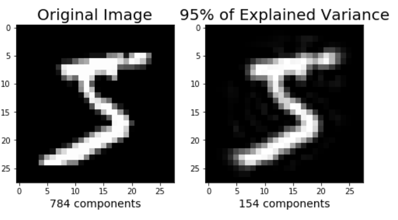
Image Reconstruction from Compressed Representation

The earlier parts of the tutorial have demonstrated using PCA to compress high dimensional data to lower dimensional data. I wanted to briefly mention that PCA can also take the compressed representation of the data (lower dimensional data) back to an approximation of the original high dimensional data. If you are interested in the code that produces the image below, check out my github.

Closing Thoughts

This is a post that I could have written on for a lot longer as PCA has many different uses. I hope this post helps you with whatever you are working on. Please let me know if you have any questions either here or on the youtube video page!