How to rewrite your SQL queries in Pandas, and more

Fifteen years ago, there were only a few skills a software developer would need to know well, and he or she would have a decent shot at 95% of the listed job positions. Those skills were:

• Object-oriented programming.
• Scripting languages.
• JavaScript, and…
• SQL.

SQL was a go-to tool when you needed to get a quick-and-dirty look at some data, and draw preliminary conclusions that might, eventually, lead to a report or an application being written. This is called exploratory analysis.

These days, data comes in many shapes and forms, and it’s not synonymous with “relational database” anymore. You may end up with CSV files, plain text, Parquet, HDF5, and who knows what else. This is where Pandas library shines.

What is Pandas?

Python Data Analysis Library, called Pandas , is a Python library built for data analysis and manipulation. It’s open-source and supported by Anaconda. It is particularly well suited for structured (tabular) data. For more information, see http://pandas.pydata.org/pandas-docs/stable/index.html.

What can I do with it?

All the queries that you were putting to the data before in SQL, and so many more things!

Great! Where do I start?

This is the part that can be intimidating for someone used to expressing data questions in SQL terms.

SQL is a declarative programming language : https://en.wikipedia.org/wiki/List_of_programming_languages_by_type#Declarative_languages.

With SQL, you declare what you want in a sentence that almost reads like English.

Pandas ’ syntax is quite different from SQL. In Pandas , you apply operations on the dataset, and chain them, in order to transform and reshape the data the way you want it.

We’re going to need a phrasebook!

The anatomy of a SQL query

A SQL query consists of a few important keywords. Between those keywords, you add the specifics of what data, exactly, you want to see. Here is a skeleton query without the specifics:

SELECT… FROM… WHERE…

GROUP BY… HAVING…

ORDER BY…

LIMIT… OFFSET…

There are other terms, but these are the most important ones. So how do we translate these terms into Pandas?

First we need to load some data into Pandas, since it’s not already in database. Here is how:

import pandas as pd

airports = pd.read_csv('data/airports.csv')
airport_freq = pd.read_csv('data/airport-frequencies.csv')
runways = pd.read_csv('data/runways.csv')

I got this data at http://ourairports.com/data/.

SELECT, WHERE, DISTINCT, LIMIT

Here are some SELECT statements. We truncate results with LIMIT, and filter them with WHERE. We use DISTINCT to remove duplicated results.

SQL	Pandas
select * from airports	airports
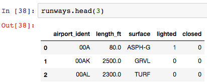
select * from airports limit 3	airports.head(3)
select id from airports where ident = 'KLAX'	airports[airports.ident == 'KLAX'].id
select distinct type from airport	airports.type.unique()

SELECT with multiple conditions

We join multiple conditions with an &. If we only want a subset of columns from the table, that subset is applied in another pair of square brackets.

SQL	Pandas
select * from airports where iso_region = 'US-CA' and type = 'seaplane_base'	airports[(airports.iso_region == 'US-CA') & (airports.type == 'seaplane_base')]
select ident, name, municipality from airports where iso_region = 'US-CA' and type = 'large_airport'	airports[(airports.iso_region == 'US-CA') & (airports.type == 'large_airport')][['ident', 'name', 'municipality']]

ORDER BY

By default, Pandas will sort things in ascending order. To reverse that, provide ascending=False.

SQL	Pandas
select * from airport_freq where airport_ident = 'KLAX' order by type	airport_freq[airport_freq.airport_ident == 'KLAX'].sort_values('type')
select * from airport_freq where airport_ident = 'KLAX' order by type desc	airport_freq[airport_freq.airport_ident == 'KLAX'].sort_values('type', ascending=False)

IN… NOT IN

We know how to filter on a value, but what about a list of values — IN condition? In pandas, .isin() operator works the same way. To negate any condition, use ~.

SQL	Pandas
select * from airports where type in ('heliport', 'balloonport')	airports[airports.type.isin(['heliport', 'balloonport'])]
select * from airports where type not in ('heliport', 'balloonport')	airports[~airports.type.isin(['heliport', 'balloonport'])]

GROUP BY, COUNT, ORDER BY

Grouping is straightforward: use the .groupby() operator. There’s a subtle difference between semantics of a COUNT in SQL and Pandas. In Pandas, .count() will return the number of non-null/NaN values. To get the same result as the SQL COUNT , use .size().

SQL	Pandas
select iso_country, type, count(*) from airports group by iso_country, type order by iso_country, type	airports.groupby(['iso_country', 'type']).size()
select iso_country, type, count(*) from airports group by iso_country, type order by iso_country, count(*) desc	airports.groupby(['iso_country', 'type']).size().to_frame('size').reset_index().sort_values(['iso_country', 'size'], ascending=[True, False])

Below, we group on more than one field. Pandas will sort things on the same list of fields by default, so there’s no need for a .sort_values() in the first example. If we want to use different fields for sorting, or DESC instead of ASC , like in the second example, we have to be explicit:

SQL	Pandas
select iso_country, type, count(*) from airports group by iso_country, type order by iso_country, type	airports.groupby(['iso_country', 'type']).size()
select iso_country, type, count(*) from airports group by iso_country, type order by iso_country, count(*) desc	airports.groupby(['iso_country', 'type']).size().to_frame('size').reset_index().sort_values(['iso_country', 'size'], ascending=[True, False])

What is this trickery with .to_frame() and .reset_index()? Because we want to sort by our calculated field ( size ), this field needs to become part of the DataFrame. After grouping in Pandas, we get back a different type, called a GroupByObject. So we need to convert it back to a DataFrame. With .reset_index(), we restart row numbering for our data frame.

HAVING

In SQL, you can additionally filter grouped data using a HAVING condition. In Pandas, you can use .filter() and provide a Python function (or a lambda) that will return True if the group should be included into the result.

SQL	Pandas
select type, count(*) from airports where iso_country = 'US' group by type having count(*) > 1000 order by count(*) desc	airports[airports.iso_country == 'US'].groupby('type').filter(lambda g: len(g) > 1000).groupby('type').size().sort_values(ascending=False)

Top N records

Let’s say we did some preliminary querying, and now have a dataframe called by_country , that contains the number of airports per country:

In the next example, we order things by airport_count and only select the top 10 countries with the largest count. Second example is the more complicated case, in which we want “the next 10 after the top 10”:

SQL	Pandas
select iso_country from by_country order by size desc limit 10	by_country.nlargest(10, columns='airport_count')
select iso_country from by_country order by size desc limit 10 offset 10	by_country.nlargest(20, columns='airport_count').tail(10)

Aggregate functions (MIN, MAX, MEAN)

Now, given this dataframe or runway data:

Calculate min, max, mean, and median length of a runway:

SQL	Pandas
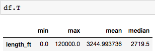
select max(length_ft), min(length_ft), mean(length_ft), median(length_ft) from runways	runways.agg({'length_ft': ['min', 'max', 'mean', 'median']})

You will notice that with this SQL query, every statistic is a column. But with this Pandas aggregation, every statistic is a row:

Nothing to worry about —simply transpose the dataframe with  .T to get columns:

JOIN

Use .merge() to join Pandas dataframes. You need to provide which columns to join on (left_on and right_on), and join type: inner (default), left (corresponds to LEFT OUTER in SQL), right (RIGHT OUTER), or outer (FULL OUTER).

SQL	Pandas
select airport_ident, type, description, frequency_mhz from airport_freq join airports on airport_freq.airport_ref = airports.id where airports.ident = 'KLAX'	airport_freq.merge(airports[airports.ident == 'KLAX'][['id']], left_on='airport_ref', right_on='id', how='inner')[['airport_ident', 'type', 'description', 'frequency_mhz']]

UNION ALL and UNION

Use pd.concat() to UNION ALL two dataframes:

SQL	Pandas
select name, municipality from airports where ident = 'KLAX' union all select name, municipality from airports where ident = 'KLGB'	pd.concat([airports[airports.ident == 'KLAX'][['name', 'municipality']], airports[airports.ident == 'KLGB'][['name', 'municipality']]])

To deduplicate things (equivalent of UNION ), you’d also have to add .drop_duplicates().

INSERT

So far, we’ve been selecting things, but you may need to modify things as well, in the process of your exploratory analysis. What if you wanted to add some missing records?

There’s no such thing as an INSERT in Pandas. Instead, you would create a new dataframe containing new records, and then concat the two:

SQL	Pandas
create table heroes (id integer, name text);	df1 = pd.DataFrame({'id': [1, 2], 'name': ['Harry Potter', 'Ron Weasley']})
insert into heroes values (1, 'Harry Potter');	df2 = pd.DataFrame({'id': [3], 'name': ['Hermione Granger']})
insert into heroes values (2, 'Ron Weasley');
insert into heroes values (3, 'Hermione Granger');	pd.concat([df1, df2]).reset_index(drop=True)

UPDATE

Now we need to fix some bad data in the original dataframe:

SQL	Pandas
update airports set home_link = 'http://www.lawa.org/welcomelax.aspx' where ident == 'KLAX'	airports.loc[airports['ident'] == 'KLAX', 'home_link'] = 'http://www.lawa.org/welcomelax.aspx'

DELETE

The easiest (and the most readable) way to “delete” things from a Pandas dataframe is to subset the dataframe to rows you want to keep. Alternatively, you can get the indices of rows to delete, and .drop() rows using those indices:

SQL	Pandas
delete from lax_freq where type = 'MISC'	lax_freq = lax_freq[lax_freq.type != 'MISC']
	lax_freq.drop(lax_freq[lax_freq.type == 'MISC'].index)

Immutability

I need to mention one important thing — immutability. By default, most operators applied to a Pandas dataframe return a new object. Some operators accept a parameter inplace=True , so you can work with the original dataframe instead. For example, here is how you would reset an index in-place:

df.reset_index(drop=True, inplace=True)

However, the  .loc operator in the UPDATE example above simply locates indices of records to updates, and the values are changed in-place. Also, if you updated all values in a column:

df['url'] = 'http://google.com'

or added a new calculated column:

df['total_cost'] = df['price'] * df['quantity']

these things would happen in-place.

And more!

The nice thing about Pandas is that it’s more than just a query engine. You can do other things with your data, such as:

• Export to a multitude of formats:

df.to_csv(...)  # csv file
df.to_hdf(...)  # HDF5 file
df.to_pickle(...)  # serialized object
df.to_sql(...)  # to SQL database
df.to_excel(...)  # to Excel sheet
df.to_json(...)  # to JSON string
df.to_html(...)  # render as HTML table
df.to_feather(...)  # binary feather-format
df.to_latex(...)  # tabular environment table
df.to_stata(...)  # Stata binary data files
df.to_msgpack(...)	# msgpack (serialize) object
df.to_gbq(...)  # to a Google BigQuery table.
df.to_string(...)  # console-friendly tabular output.
df.to_clipboard(...) # clipboard that can be pasted into Excel

• Plot it:

top_10.plot(
    x='iso_country', 
    y='airport_count',
    kind='barh',
    figsize=(10, 7),
    title='Top 10 countries with most airports')

to see some really nice charts!

• Share it.

The best medium to share Pandas query results, plots and things like this is Jupyter notebooks (http://jupyter.org/). In facts, some people (like Jake Vanderplas, who is amazing), publish the whole books in Jupyter notebooks: https://github.com/jakevdp/PythonDataScienceHandbook.

It’s that easy to create a new notebook:

$ pip install jupyter
$ jupyter notebook

After that: 

• navigate to localhost:8888
• click “New” and give your notebook a name
• query and display the data
• create a GitHub repository and add your notebook (the file with  .ipynb extension).

GitHub has a great built-in viewer to display Jupyter notebooks with Markdown formatting.

And now, your Pandas journey begins!

I hope you are now convinced that Pandas library can serve you as well as your old friend SQL for the purposes of exploratory data analysis — and in some cases, even better. It’s time to get your hands on some data to query!

Republished from https://codeburst.io/how-to-rewrite-your-sql-queries-in-pandas-and-more-149d341fc53e.