Timeline of Transfer Learning Models

In this post, we will have a timeline of some of the most powerful transfer learning models for image classification and how they’ve evolved over the last few years. In Transfer Learning, we can use pre-trained models and add a few densely connected layers in order to recognize objects from a new dataset. In the documentation of Keras, we can find some pre-trained models that can be imported such as VGG, ResNet and Inception. Before getting into more details of each model, let’s check where those models come from. Those models are from a yearly competition called ImageNet.

ImageNet

ImageNet is a large visual database designed for researching visual object recognition software. The project manually annotated more than 14 million images to indicate objects into more than 20,000 categories. Since 2010, the ImageNet project has launched an annual software competition called ImageNet’s Large Scale Visual Identity Challenge (ILSVRC), in which software programs compete to properly classify and detect objects and scenes. The challenge uses a subset of the original dataset with 1.2 million images for training as input and one thousand categories as output.

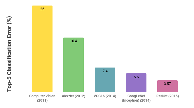
Over the last few years, the average error has been constantly decreasing. Since 2012 there was a major shift from classical computer vision techniques to Deep Learning. AlexNet was the first winner to use Deep Learning techniques and its error decreased more than 10 percent when compared to the winner of the previous year using computer vision. Let’s discuss some of those models further.

2012 — AlexNet

In 2012, AlexNet was able to outperform classical computer vision models by a large gap of 10%. It was the first time a deep neural network was the winner for this type of competition and since then, deep learning became the standard approach for image classification problems. It is composed of five pairs of convolutional layers followed by two pairs of fully connected layers, as shown in Figure 2. Due to computation limitations at that time, the training was done on two GPUs which is the reason why their network is split into two pipelines.

Figure 2: AlexNet Model

AlexNet helped to spread and standardize the following practices:

• ReLu (Rectified Linear Unit) as the default activation function of hidden layers instead of a Tanh or Sigmoid which was the earlier standard. The advantage of ReLu is that it trains since its derivative is constant for positive values. This also helps with the vanishing gradient problem.
• Dropout layer after each Fully Connected layer in order to decrease overfitting. It randomly switches off the activation of a portion of the units given as a parameter (its default is 50%). The reason it works is that dropout helps the network to develop independent features by forcing units to learn from different subsets from the previous units.

In 2013 the winner was ZFNet. Its architecture was similar to AlexNet with improvements in the numbers of filters and hyperparameters. In general, it was the same idea.

2014 — VGG and GoogLeNet

In 2014 there was another jump in performance thanks to deeper networks. From eight layers in the previous year, now in 2014, there were two close winners, VGG and GoogLeNet, with 19 and 22 layers respectively. So let’s first look at VGG in a little bit more detail.

VGG

VGG which is from VGG Group, Oxford, had two versions, one with 16 layers and another 19 layers. It was composed of five sets of convolutional layers followed by maxpooling each. The convolutional layers used 3 by 3 kernel-sized filters instead of 11 which was used by AlexNet which helped to decrease the number of parameters while still capturing features from the previous layer. It is a popular model to be used as a starting point due to its simplicity. However, the model is quite large in the number of parameters and heavy to be loaded in memory. At that time, models with about 20 layers were considered very deep models due to problems with the vanishing gradient problem. As we will see soon, the invention of batch normalization and residual networks made possible to train models with much more layers.

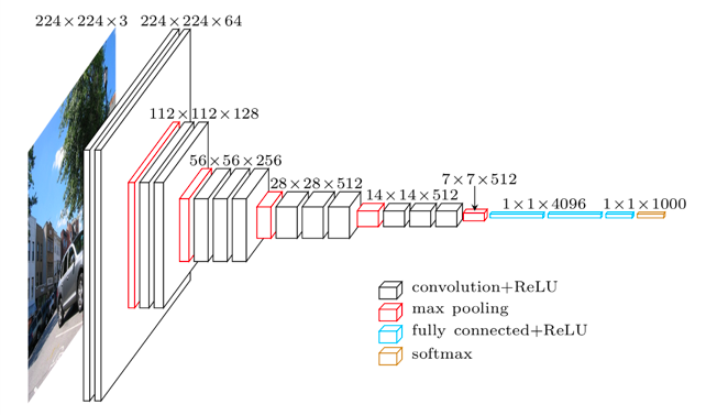VGG Architecture (Image Credits)

VGG helped to spread and standardize the following practices:

• Convolutional filters with size 3x3

GoogLeNet (Inception)

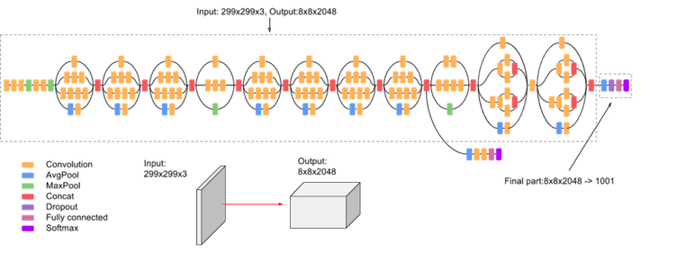
GoogLeNet, also known as Inception, has 12 times fewer parameters than AlexNet and is the ILSVRC 2014 classification winner. It is composed of 22 layers. Its main key point is that they designed a module called inception in order to handle the problem of computational efficiency. The inception module stacks a lot of those modules on top of each other to compute the network more efficiently. They’re basically applying several different kinds of filter operations in parallel on top of the same input coming into this same layer. Then they concatenate all these filter outputs together depth-wise, and so then this creates one tenser output at the end that is going to pass on to the next layer. Another point about the module is the bottleneck layer which is one by one kernel-sized filters. They reduce the computational complexity by reducing the number of filters. Finally, there are no fully connected layers in the output of the network after the convolutional filters. Instead, they use a global average pooling layer which allows the usage of fewer parameters.

GoogLeNet helped to spread and standardize the following practices:

• Inception modules with different operations in parallel and concatenation of them depth-wise.
• Global Average Pooling instead of fully-connected layers at the end after the convolutional filters in order to reduce complexity.

2015 — ResNet

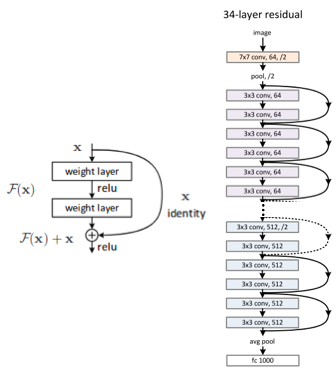ResNet Model (Image Credits)

ResNet was the winner of 2015's competition with a model with 152 layers. They were able to get 3.57% top 5 error in the classification accuracy which is better than human performance. This drastic increase in the number of layers was possible because of two main key points: the usage of what they call residual connections and also the usage of batch normalization for handling the gradient flow in the earlier layers. The residual connections are connections with identity mapping of previous layers. The intuition behind those connections was that they noticed that very deep models were performing worse than shallow networks due to the vanishing gradient problem. As a solution, they hypothesized that deeper models should perform at least as good as shallower models. This was possible by using connections with identity mapping of previous layers skipping some layers ahead making the network equivalent to a shallower model but also with the potential of learning more complex decision boundaries. They also use global average pooling instead of flattening followed by fully connected layers. Another major point in the network is the usage of batch normalization, which avoids that the propagation of gradients either explode or tend to zero.

ResNet helped to spread and standardize the following practices:

• Residual connections in order to make the model at least as good as shallower networks but also with the potential of becoming superior.
• Batch Normalization after every convolutional layer for improving the stability, speed, and performance of the training process.

Summary

In summary, we’ve seen different kinds of CNN Architectures. We looked at four of the main architectures that you’ll see in wide usage. AlexNet, one of the early, very popular networks. VGG and GoogleNet which are still widely used. But ResNet is kind of taking over as the thing that you should be looking most when you can. There’s a trend toward the design of how do we connect layers, skip connections, what is connected to what, and also using these to design your architecture to improve gradient flow. The following key points of each model are mentioned:

• AlexNet: ReLu as activation function and Dropout after each FC layer.
• VGG: Most common architecture what we’ll usually see, with max pooling, 3x3 kernel-sized filters, convolutional filters followed by fully connected layers.
• Inception/GoogLeNet: Inception modules with different operations in parallel; global average pooling instead of fully-connected layers; ‘bottleneck’ layers with one by one kernel-sized filters to reduce the depth of convolutional layers.
• ResNet: Residual connections in order to make the model equivalent to shallower networks; batch normalization for improving performance.