Naive Bayes Classifier: A Geometric Analysis of the Naivete. Part 1

The curse of dimensionality is the bane of all classification problems. What is the curse of dimensionality? As the the number of features (dimensions) increase linearly, the amount of training data required for classification increases exponentially. If the classification is determined by a single feature we need a-priori classification data over a range of values for this feature, so we can predict the class of a new data point. For a feature $x$ with 100 possible values, the required training data is of order O(100). But if there is a second feature $y$ as well that is needed to determine the class, and $y$ has 50 possible values, then we will need training data of order O(5000) – i.e. over the grid of possible values for the pair "$x,y$". Thus the measure of the required data is the volume of the feature space and it increases exponentially as more features are added.

But is this always this bad? Are there some simplifying assumptions we can make to decrease the amount of data required, even while keeping all the features? In the above example we said we needed training measurements of order O(5000). But naive bayes classifier needs measurements of order only O(150) – i.e. just a linear increase, not an exponential one! That is fantastic but we know there is no free lunch and naive bayes classifier should be making some simplifying (naive?) assumptions. That is the purpose of this post – examine the impact of naivete in the naive bayes classifier that allows it to side-step the curse of dimensionality. On a practical note, we do not want the algebra to detract us from appreciating what we are after, so we stick to 2 dimensions $x,y$ and 2 classes $C_1$ and $C_2$.

Decision Boundary

Decision boundary is a curve in our 2-dimensional feature space that separates the two classes $C_1$ and $C_2$. In Figure 1, the zone where y–f(x)>0 indicates class $C_1$ and y–f(x)<0 indicates $C_2$. Along the decision boundary $y=f(x)$ the probability of belonging to either class is equal. Equal probability of either class is the criterion to obtain the decision boundary.

Figure 1. The decision boundary separates the two classes $C_1$ and $C_2$ in the feature space. For points on the decision boundary, the probability of belonging to either class is the same.

The objective of this post is to analyse the impact of nonlinearities in the decision boundary and the coupled issues that arise from unbalanced class sizes. The overall outline for this post is as follows.

1. Pick an exact functional form $y=f(x)$ for the true decision boundary.
2. Obtain a closed-form solution to the decision boundary as predicted by  naive bayes classifier
3. Analyse the impact of class sizes on the predictions
4. Obtain the asymptotic behavior when one of the classes overwhelms the other
5. Repeat 1 thru 4 when $f(x)$ is linear and nonlinear.

The content of the post is somewhat academic as with real data we do not know the true decision boundary, have to deal with data noise, and do not know which features are actually responsible for classification we seek etc… But the point here is to understand the impact of naivete assumption in an idealized setting so we would be better equipped to apply and interpret the naive bayes classifier for real data.

1. Naive Bayes Classification

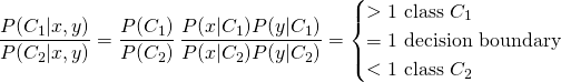
Naive bayes classification is based on Bayes rule that relates conditional and marginal probabilities. It is well described in literature so we simply write the equations down for a 2 class ($C_1$ and $C_2$) situation with 2 features $x,y$.

(1)  

For any new measurement $x,y$ we would compute $P(C_1|x,y)$ and $P(C_2|x,y)$, as per Equation 1 and pick the class with the larger value. As the denominator is the same it is easier to just compute their ratio so we do not have to evaluate $P(x,y)$

$P(C_i)$ is the probability for any measurement to fall into the class $C_i$. It is computed easily enough from the training data as the relative abundance of $C_i$ samples. It is the computation of $P(x,y|C_i)$ that is fraught with the challenge of data requirements we talked about. To do it right we need to estimate the joint probability distribution of $x,y$ in each class $C_i$ and that requires training data on a grid of $x,y$ values. That is where the naive part of naive bayes comes in to alleviate the curse of dimensionality.

1.1 The Naive Assumption

If the features $x,y$ were to be uncorrelated, given the class $C_i$ then the joint probability distribution would simply be the product of individual probabilities. That is

(2)  

If we make this assumption then we only need to estimate $P(x|C_i)$ and $P(y|C_i)$ separately. And that only requires training data on the range of $x$ and on the range of $y$ – not on a grid of $x,y$ values. Using Equation 2 in Equation 1 we get the ratio of the class probabilities for a new $x,y$ measurement and its class assignment thereof to be as follows

(3)  

While the naive assumption of uncorrelated features simplifies things, its validity is open to question. If for example $xy<1$ in a class, then the probability of finding large $x$ values will be higher when $y$ is small, and lower when $y$ is large. In fact the probability of finding the measurement $x$=0.9,$y$=1.1 in this class will be unity, whereas it would be zero for the measurement $x$=0.9,$y$=1.2. Clearly, the probability distributions of $x$ and $y$ will not in general be independent of each other and making the naive assumption of independence can lead to incorrect class assignment for new data.

1.2 Deriving $P(x|C_i)$ and $P(y|C_i)$

If we can obtain $P(x|C_i)$ and $P(y|C_i)$ as functions of $x,y$ then we have the ratio in Equation 3 as a function of $x,y$.

Figure 2. Deriving the naive bayes probabilities, given a true decision boundary $y=f(x)$. To keep the algebra simple, the function $f(x)$ is taken to have a simple inverse $y=f^{-1}(x)$. The fractional areas of the rectangular strips in a class are indicative of the probability.

Consider Figure 2 where the true decision boundary $y=f(x)$, splits the feature space into two classes. To keep the algebra at bay, we further take $f$ to be explicitly invertible so we can write $x=f^{-1}(y)$.The a-priori probability of a class is proportional to its overall size – area in this case.

(4)  

To compute $P(x|C_i)$ imagine that we discretized the x-axis and picked a small rectangular strip of width δx around $x$ as shown in Figure 2. The area of the strip in class $C_i$ divided by the class area $A_i$ would be the probability $P(x|C_i). Likewise for the probability $P(y|C_i)$

(5)  

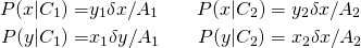
The longer $x_1$ is, the higher the probability of $P(y|C_1)$ would be. Likewise a larger $y_2$ implies a higher probability for $P(x|C_2)$ and so forth. Once we appreciate this, the rest is simply geometry and algebra. Combining Equations  4 and 5 with naive bayes classification in Equation 3, we get:

(6)  

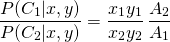
The locus of $x,y$ for which the ratio above equals unity is the decision boundary as predicted by the naive bayes classifier.

(7)  

Figure 3. For a point on a linear decision boundary, a geometric proof that: (a) $x_1y_1 = x_2 y_2$ in case of balanced classes and (b) $x_1 y_1 \neq x_2 y_2$ when classes are unbalanced.

For an intuitive understanding of Equation 7 consider the case of a linear decision boundary with equal/unequal class sizes in Figure 3. When class sizes are equal as in Figure 3.1 the decision boundary would be the diagonal, and for every point on the diagonal, the area of the rectangle ABOC equals the area of the rectangle ODEF. But that is nothing but a statement about the equality of $x_1y_1$ and $x_2y_2$ for any point on the diagonal.Thus as per Equation 7 the decision boundary predicted by naive bayes will match the diagonal – the true decision boundary. In Figure 3.2 however, the class sizes are not the same and the areas of these two rectangles do not have to be equal for every point on the separation boundary. So we cannot expect naive bayes to yield the true decision boundary even in the linear case when the class sizes are not the same. We shall verify this again analytically in the next section.

That completes our general method for deriving the decision boundaries as predicted by naive bayes. For the remainder of the post we choose different functional forms for the true decision boundary $f(x)$ and contrast that with what we get from naive bayes.

2. A Linear Decision Boundary

We start with the linear case in Figure 4 where a straight line $y = qx/a$ separates the two classes in a rectangular feature space. When $q$ equals $b$ we get balanced classes.

Figure 4. Evaluating $x_1$, $y_1$, $x_2$ and $y_2$ for a linear decision boundary $y=qx/a$

The class areas $A_1$, $A_2$ and the lengths $x_1, x_2, y_1$, and $y_2$ follow directly from the geometry. Using them in Equation 7 and simplifying we get the decision boundary as predicted by naive bayes to be a hyperbola.

(8)  

With the closed-form solution in hand for the predicted separation boundary, we can look at the impact of class size and asymptotics thereof when the size of class $A_1$ keeps increasing while $A_2$ stays constant. This is achieved through increasing $b$ while holding $a$ and $q$ constant.

2.1 Balanced classes. $A_1$ = $A_2$

When $b=q$, the class sizes would be equal and the separation boundary reduces to:

(9)  

which is the true decision boundary. That is, naive bayes classification will have no error when the classes are separated by straight line and have the same size. This is a rigorous proof of the same geometric argument made in Figure 3.

2.2 Unbalanced classes. Increasing $A_1$ and constant $A_2$

Figure 5 shows the predicted decision boundaries as $b$ is increased (i.e. we drag the top-boundary of the feature space), thus increasing $A_1$ while holding $A_2$ constant. In all the cases the naive bayes predictions start off favoring class $C_2$ (the predicted boundaries are above the true boundary – meaning a preference to classify a true $C_1$ measurement as $C_2$) for smaller $x$ and switching over to prefer class $C_1$ as $x$ increases. It is interesting however that they all switch over at the same point on the true decision boundary.

2.2.1 The switch over point

The switch over point $(x^*, y^*)$ is the intersection of the true decision boundary and the predicted decision boundary. Using $y=qx/a$ in Equation 8 and simplifying we get,

(10)  

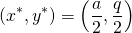
Figure 5. Linear decision boundary. Naive bayes classifier predicts a hyperbola as the class boundary. Only when the classes are balanced does the prediction match the prescribed boundary $y=x$

The coordinates of this point are independent of $b$ – the only variable across the different curves. Hence they all intersect the true boundary at the same point.

2.2.2 The asymptotic boundary: $A_1 \rightarrow \infty$

As $b$ increases, the ratio $A_1/A_2$ increases. In the limit as $b$ goes to infinity, we get the asymptotic prediction boundary $y_s(x)$.

(11)  

3. A Nonlinear Decision Boundary

We now consider the case in Figure 6 where a parabolic decision boundary $y=x^2$ separates the two classes.

Figure 6. Evaluating $x_1, y_1, x_2$, and $y_2$ for a nonlinear decision boundary $y=x^2$

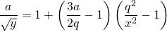
Once again the expressions for $x_1, y_1, x_2$, and $y_2$ as functions of $x,y$ follow directly from the geometry. Applying Equation 7 and simplifying we get $y$ as a fourth order function of $x$ for the predicted decision boundary

(12)  

3.1 Effect of increasing $A_2$ and constant $A_1$

Figure 7. Nonlinear decision boundary. The naive bayes prediction does not match the true boundary even in the case of balanced classes.

Figure 7 shows the predicted decision boundary Vs the true boundary as the class size $A_2$ is varied while holding $A_1$ constant. This is simply done by dragging the right-boundary of the feature space, i.e changing $a$.

Here are a few quick observations that are in contrast with the linear case.

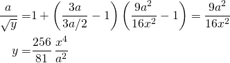
• Even in the case of balanced classes ($A_1/A_2=1$ i.e. $a=4q/3$), the predicted boundary does NOT match the true boundary. This is unlike the linear case as we have seen earlier. Using $q=3a/4$ in Equation 12 we get:

(13)  

• For small $x$ the prediction favors $C_1$ over $C_2$ (the predicted boundry starts off below the true boundary in all cases) but switches over to prefer $C_2$ for larger $x$.
• When $A_2$ is small the predicted boundary is mostly under the true boundary over the range of $x$. For larger $A_2$ the predicted boundary gets steeper and intersects the true boundary earlier and earlier. Thus unlike in the linear case they intersect the true boundary at different points.
• Even while they intersect the true boundary at different points, it is interesting to note that they all intersect each other at a single point. That can be proved of course. The only variable across the different curves is $a$. So all we have to is to find the point of intersection for two predicted boundaries and show that it is independent of $a$. Consider two such boundaries for $a_1$ and $a_2$. Using Equation 12 at the point of their intersection and simplifying we get,

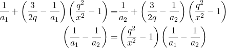
yielding the intersection point to be independent of $a$ thus proving the observation.

(14)  

3.2 Asymptotic boundary: $A_2 \rightarrow \infty$

As $a$ increases, the area $A_2$ increases. In the limit as $a$ goes to infinity, we get the asymptotic prediction boundary $y_s(x)$.

(15)  

4. Next Steps

We have derived closed-form solutions to the decision boundaries predicted by naive bayes classifier, when the true decision boundary is known between 2 classes with 2 features. We picked simple linear and nonlinear boundaries and evaluated the impact of class sizes and asymptotics thereof when one class overwhelms the other. The next steps are as follows.

• Obtain the confusion matrix as a function of class size ratio while the total size is remains constant. For example as we vary $q$ from 0 to 1 in the Figure 4, the ratio $A_1/A_2$ goes from $\infty$ to 0 while $A_1+A_2$ stays constant at $ab$. The performance of naive bayes classifier gauged via the various metrics coming off of the confusion matrix is of interest in this case.
• Simulate the Gaussian Naive Bayes algorithm as implemented in SciKit to evaluate the additional errors introduced by the gaussian approximation to probability.
• Evaluate naive bayes predictions against other competing classifiers such as logistic regression, neural nets etc…

As this post is getting too long so will take up the above and more in the next post in this series.