
Mastering data structures in Ruby — AVL Trees
Binary search trees , or BTS s for short, are data structures designed to perform fast lookups on large datasets. The subject of this post is AVL trees , a special kind of self-balancing BST named after its creators Adelson-Velskii and Landis where the height difference between the left and right subtrees (the balance factor) is always in the range (-1..1) giving us O(log2 n) lookups.
On AVL trees nodes arranged in descendant order, and they can’t contain duplicate keys. These properties are important because most of its methods rely on them.
Let’s start by looking at how lookups work.
How lookups work
On this data structure lookups are top-down recursive-descendant operations; which means that they start from the root node and move all the way down until they find the key they are looking for or run out of nodes.
Of course, inspecting the whole tree would be prohibitively expensive, but since nodes are guaranteed to be sorted, we don’t have to do that. We start from the top, descending left or right based on how our key compares to the current node’s.
If the key of the current node is higher than the key we are looking for, we move to the left; otherwise, we go to the right. In any case, we have to repeat this operation until we find the key we are looking for, or we get to the end of the branch (EOB).
An AVL Tree looks something like:
          4
         / \
        /   \
       2     6
      / \    / \
     1   3  5   9
                / \
               7  11
Now let’s say we want to find the number 5.
Starting from the root node, the way to go would be:
1. Is 5 == 4?No

2. Is 5 < 4?No. Move right.

3. Is 5 == 6?No

4. Is 5 < 6?Yes. Move left.

5. Is 5 == 5Yes. We found it!
*Note: To simplify the lookup process I’ve omitted the check for “end of the branch”.
So, to find the number 5 we only need 2 traversals from the root; the same operation on a singly linked list would require 5.
For a small number of elements it doesn’t look like a big difference; however, what is interesting about AVL trees is that lookups run O(log2 n) time; which means that they get exponentially better than linear search as the dataset grows.
For instance, looking for an element out of a million on a singly linked list could require up to 1,000,000 traversals. The same operation on AVL trees would require roughly 20!
How inserts work
Inserts and searches are tightly coupled operations. So, now that we know how searches work, let’s take a look at inserts. Or better yet, rotations , which are the interesting bits of inserts.
Rotation is a mechanism to rearrange parts of a tree to restore its balance without breaking these properties:
- left’s key < parent’s key
- parent’s key < right’s key
Once the rotation is completed, the balance factor of all nodes must be in the balanced range (-1..1).
Depending on the location of the node that puts the tree into an unbalanced state, we have to apply one of these rotations (LL, LR, RR, RL). Let’s take a look at each one of them.
LL (left-left)
Suppose we want to add the number 1 to the following subtree:
       /
      6
     / \
    3   7
   / \
 2     4
/
x
By following the rules we use for lookups operations, we descend from top to bottom, moving left or right, until we find an empty spot. In this case, that spot will be the left subtree of the node that contains the number 2. Once we are there, we insert the new node.
       /
      6
     / \
    3   7
   / \
  2   4
 /
1
So far, so good; but now we have a problem. After inserting the new node, the balance factor of the subtree’s root node (6) went to +2, which means that we must balance the tree before going on.
To know which kind of rotation we have to apply, we can follow the path from the unbalanced node to the node we just added. Let’s annotate the tree to visualize this path:
         /
        6
       / \
  (L) 3   7
     / \
(L) 2   4
  /
1
In this case, the node is rooted at the left subtree of the left subtree of the unbalance node; hence, we have to do a left-left rotation (LL).
LR (left-right)
Now let’s take a look at a left-right rotation (LR). A rotation we have to apply when the new node lies on the right subtree of the left subtree of the node that got unbalanced.
In the following three that rotation will take place if we have to insert the number 5 into the tree.
     /
    6
   / \
  3   7
 / \
2   4
     \ 5 (*)
RR (right-right)
The third kind of rotation is the right-right rotation (RR). This rotation happens when the new node is on the right subtree of the right subtree of the unbalanced node. For instance, that will happen if we insert the number 11 into the following tree.
   /
  4
 / \
3   6
    / \
   5   9
         \ 11 (*)
RL (right-left)
The last kind of rotation is the right-left rotation (RL). A rotation that happens when the new node lies on the right subtree of the left subtree of the node that got unbalanced.
After inserting the number 4 in the following tree, we must perform an RL rotation to restore its balance.
    /
   2
  / \
 1   6
    / \
   5   9
  /
4 (*)
Interface for AVL trees
The public API for this data structure is straightforward. It only has four methods and no attributes.
Methods
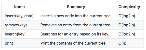
AVL Tree’s public methods.
Implementation details
As opposed to what we did in previous posts, this time we are going to focus the private methods of the data structure. By doing so, we will be covering important details that otherwise would be unnoticed.
Let’s start by looking at how nodes are represented on the AVL tree.

AVL Node’s attributes.
*Note: To make the code easy to follow I’m not going to use the binary tree we built on the previous post. I did a prototype using that code, and the result wasn’t ideal; AVL trees have much logic that mangled with B-Trees looked a bit clumsy to me. So I think this time it will be better if we start from scratch.
Insert
Adds a new node to the tree and reset its root. This method relies on insert_and_balance that takes care of applying the right rotations to keep the tree in balance.
The complexity of this method is O(log2 n).
def insert key, data = nil
  @root = insert_and_balance(@root, key, data)
end
Insert And Balance
This method looks recursively to find the right spot for the given key. Once the spot is found and the new node is inserted, it calls the balance method to ensure that the tree remains balanced.
The complexity of this method is O(log2 n).
def insert_and_balance node, key, data = nil
  return Node.new key, data unless node

  if (key < node.key)
    node.left = insert_and_balance(node.left, key, data)
  elsif(key > node.key)
    node.right = insert_and_balance(node.right, key, data)
  else
    node.data = data
    node.deleted = false
  end

  balance(node)
end
Balance
This method balances the subtree rooted at the specified node. This method is probably the most complex in this data structure because it’s responsible for selecting the right kind of rotation based on the “heaviness” of the tree.
A tree is considered left-heavy is its balance factor is higher than 1 or right-heavy if it’s lower than -1.
The best way to follow this method is by looking at the ASCII representations of each use-case in previous sections.
The complexity of this method is O(log2 n).
def balance node
  set_height node
  if (height(node.left) - height(node.right) == 2)
    if (height(node.left.right) > height(node.left.left))
      return rotate_left_right(node)
    end
    return rotate_right(node)
  elsif (height(node.right) - height(node.left) == 2)
    if (height(node.right.left) > height(node.right.right))
      return rotate_right_left(node)
    end
    return rotate_left(node)
  end
  return node
end
Remove
This method finds the node to be removed and marks it as deleted. Performance wise, this is a neat way to handle deletions because the structure of the tree doesn’t change, and so we don’t have to balance it after the node is removed.
This technique is called “lazy” removal because it doesn’t do much work.
The complexity of this method is O(log2 n).
def remove key
  search(key)&.deleted = true
end
Search
This method starts a top-down recursive descendant search from the current tree’s root node.
The complexity of this method is O(log2 n).
def search key
  node = search_rec @root, key
  return node unless node&.deleted
end
Search Rec
Searches for a key in the subtree that starts at the provided node. This method starts the search at a given node and descends (recursively) moving left or right based on the key’s values until it finds the key or gets to the end of the subtree.
The complexity of this method is O(log2 n).
def search_rec node, key
  return nil unless node
  return search_rec(node.left, key) if (key < node.key)
  return search_rec(node.right, key) if (key > node.key)
  return node
end
Set height
This method calculates and sets the height for the specified node based on the heights of their left and right subtrees.
The complexity of this method is O(1).
def set_height node
  lh = height node&.left
  rh = height node&.right
  max = lh > rh ? lh : rh
  node.height = 1 + max
end
Rotate right
This method performs a right rotation.
The complexity of this method is O(1).
def rotate_right p
  q = p.left
  p.left = q.right
  q.right = p
  set_height p
  set_height q
  return q
end
Rotate Left
This method performs a left rotation.
The complexity of this method is O(1).
def rotate_left p
  q = p.right
  p.right = q.left
  q.left = p
  set_height p
  set_height q
  return q
end
Rotate Left Right
This method points the left subtree of the given node to the result of rotating that subtree to the left and then rotates the specified node to the right. The last rotation it’s also its return value.
The complexity of this method is O(1).
def rotate_left_right node
  node.left = rotate_left(node.left)
  return rotate_right(node)
end
Rotate Right Left
This method points the right subtree of the given node to the result of rotating that subtree to the right and then rotates the specified node to the left. The last rotation it’s also its return value.
The complexity of this method is O(1).
def rotate_right_left node
  node.right = rotate_right(node.right)
  return rotate_left(node)
end
This method prints the contents of a tree.
Since it has to visit all nodes in the tree, the complexity of this method is O(n).
def print
  print_rec @root, 0
end

def print_rec node, indent
  unless node puts "x".rjust(indent * 4, " ")
  return
end

puts_key node, indent
  print_rec node.left, indent + 1
  print_rec node.right, indent + 1
end

def puts_key node, indent
  txt = node.key.to_s
  if node.deleted txt += " (D)"
    puts txt.rjust(indent * 8, " ")
  else
    puts txt.rjust(indent * 4, " ")
  end
end
When to use binary search trees
Binary search trees work well when we have to handle large datasets in applications where the read/write ratio is 10 > 1 or more. If the volume of data is small or the read/write ratio is even is better to use hash tables or even linked lists instead.
I recently used this data structure to implement the internal storage for a spreadsheet component, and it worked like a charm.
This was a rather long post that I hope you enjoy it!
You can get the source code from here.
Next time, Graphs. Stay tuned.
Thanks for reading! See you next time.
PS: If you are a member of the Kindle Unlimited program, you can read a bit polished version of this series_ for free on your Kindle device.

Data Structures From Scratch — Ruby Edition.