Convolution Neural Network (CNN): Introduction

Convolution Neural Network:  When it comes to Machine Learning, Artificial Neural Networks perform really well. Artificial Neural Networks are used in various classification task like images, audios, words, etc. Different types of Neural Networks are used for different purposes, for example for predicting the sequence of words we use Recurrent Neural Networks, more precisely a LSTM, similarly for image classification we use Convolution Neural Network. In this blog, we are going to build basic building block for CNN.

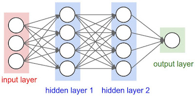
Before diving into the Convolution Neural Network, let us first revisit some concepts of Basic Neural Network. In a regular Neural Network there are three types of layers:

1. Input Layers:  It’s the layer in which we give input to our model. The number of neurons in this layer is equal to total number of features in our dataset (number of pixels incase of an image).
2. Hidden Layer:  The input from Input layer is then fed into the hidden layer. There can be many hidden layers depending on our model and size of dataset. Each hidden layers can have different number of neurons which are generally greater than the number of features. The output from each layer is computed by matrix multiplication of output of the previous layer with learnable weights of that layer and then by addition of learnable biases followed by activation function which makes the network nonlinear.
3. Output Layer:  The output from the hidden layer is then fed into a logistic function like sigmoid or softmax which converts the output of each class into probability score of each class.

The data is then fed into the model and output from each layer is obtained this step is called feedforward, we then calculate the error using an error function, some common error functions are cross entropy, square loss error, etc. After that, we train our model using various optimizers. Gradient Descent is the most important technique and the foundation of how we train and optimize Intelligent Systems. Some popular variant of gradient descent are Adagrad, AdaDelta, Adam, etc. This step is called Backpropagation which is basically used to minimize the loss.

Here’s the basic python code for a neural network with random inputs and two hidden layers.

activation = lambda x: 1.0/(1.0 + np.exp(-x)) # sigmoid function
input_layer = np.random.randn(3, 1)
hidden_1 = activation(np.dot(W1, input_layer) + b1)
hidden_2 = activation(np.dot(W2, hidden_1) + b2)
output = np.dot(W3, hidden_2) + b3

W1,W2,W3,b1,b2,b3  are learnable weights of the model.

Image source: cs231n.stanford.edu

Convolution Neural Networks or covnets are neural networks that share their parameters. Imagine you have an image. It can be represented as a cuboid having its length, width (dimension of the image) and height (as image generally have red, green, and blue channels).

Now imagine taking a small patch of this image and running a small neural network on it, with say, k outputs and represent them vertically. Now slide that neural network across the whole image, as a result, we will get another image with different width, height, and depth. Instead of just R, G and B channels now we have more channels but lesser width and height. his operation is called Convolution. If patch size is same as that of the image it will be a regular neural network. Because of this small patch, we have fewer weights.

Image source: Deep Learning Udacity

Now let’s talk about a bit of mathematics which is involved in the whole convolution process.

• Convolution layers consist of a set of learnable filters (patch in the above image). Every filter has small width and height and the same depth as that of input volume (3 if the input layer is image input).
• For example, if we have to run convolution on an image with dimension 34x34x3. Possible size of filters can be axax3, where ‘a’ can be 3, 5, 7, etc but small as compared to image dimension.
• During forward pass, we slide each filter across the whole input volume step by step where each step is called stride (which can have value 2 or 3 or even 4 for high dimensional images) and compute the dot product between the weights of filters and patch from input volume.
• As we slide our filters we’ll get a 2-D output for each filter and we’ll stack them together and as a result, we’ll get output volume having a depth equal to the number of filters. The network will learn all the filters.

Layers used to build ConvNets

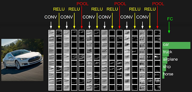
A covnets is a sequence of layers, and every layer transforms one volume to another through differentiable function.
Types of layers:
Let’s take an example by running a covnets on of image of dimension 32 x 32 x 3.

1. Input Layer:  This layer holds the raw input of image with width 32, height 32 and depth 3.
2. Convolution Layer:  This layer computes the output volume by computing dot product between all filters and image patch. Suppose we use total 12 filters for this layer we’ll get output volume of dimension 32 x 32 x 12.3. Activation Funtion Layer:  This layer will apply element wise activation function to the output of convolution layer. Some common activation functions are RELU: max(0, x), Sigmoid: 1/(1+e^-x), Tanh, Leaky RELU, etc. The volume remains unchanged hence output volume will have dimension 32 x 32 x 12.
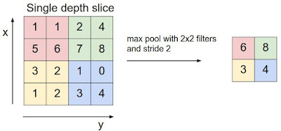
3. Pool Layer:  This layer is periodically inserted in the covnets and its main function is to reduce the size of volume which makes the computation fast reduces memory and also prevents from overfitting. Two common types of pooling layers are  max pooling  and  average pooling. If we use a max pool with 2 x 2 filters and stride 2, the resultant volume will be of dimension 16x16x12.
   
4. Fully-Connected Layer:  This layer is regular neural network layer which takes input from the previous layer and computes the class scores and outputs the 1-D array of size equal to the number of classes.