
Unfolding Naïve Bayes from Scratch !

Photo Credits : Mikito Tateisi on Unsplash
Unfolding Naïve Bayes from Scratch! Take-1 🎬
W hether you are a beginner in Machine Learning or you have been trying hard to understand the Super Natural Machine Learning Algorithms and you still feel that the dots do not connect somehow, this post is definitely for you!
My Sole Purpose of Writing this Blog Post
I have tried to keep things simple and in plain-English. The sole purpose is to deeply and clearly understand the working of a well know Text Classification ML Algorithm (Naïve Bayes) without being trapped in the gibberish mathematical jargon that is often used in the explanation of ML Algorithms which obviously lands you nowhere except for being relying on ML API’s with almost zero understanding of how the things actually work!
Who is the Target Audience?
ML beginners who are seeking in depth yet understandable explanation of ML Algorithms from scratch
Outcome of this Tutorial
A complete clear picture of the Naïve Bayes ML Algorithm with all its mysterious mathematics demystified plus a concrete step taken forward in your ML voyage! Cheers 😃
Defining The Roadmap….. 🚵
Milestone # 1 : A Quick Short Intro to The Naïve Bayes Algorithm
Milestone # 2 : Training Phase of The Naïve Bayes Model
The Grand Grand Grand Milestone # 3 : The Testing Phase —Where Prediction Comes into the Play!
Milestone # 4 : Digging Deeper into the Mathematics of Probability
Milestone # 5 : Avoiding the Common Pitfall of The Underflow Error!
Milestone # 6 : Concluding Notes….
A Quick Short Intro to The Naïve Bayes Algorithm
Naive Bayes is one of the most common ML algorithms that is often used for the purpose of text classification. If you have just stepped into ML, it is one of the easiest classification algorithms to start with. Naive Bayes is a probabilistic classification algorithm as it uses probability to make predictions for the purpose of classification.
So, if you are looking forward to take a step forward into Machine Learning Voyage, Naïve Bayes Classifier is definitely your next stop!
Milestone # 1 Achieved 👍
Training Phase of The Naïve Bayes Model
Let’s say, there is a restaurant review, “Very good food and service!!!”, and you want to predict that whether this given review implies a positive or a negative sentiment. To do this, we will first need to train a model ( that essentially means to determine counts of words of each category) on a relevant labelled training data set and then this model itself will be able to automatically classify such reviews into one of the given sentiments against which it was trained for. Assume that you are given a training dataset which looks like something below (a review and it’s corresponding sentiment):
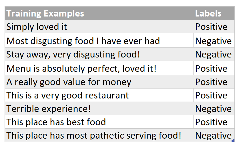
Labelled Training Dataset
A Quick Side Note : Naive Bayes Classifier is a Supervised Machine Learning Algorithm
So how do we begin?
Step # 1 : Data Preprocessing
As part of the preprocessing phase (which is not covered in a detail in this post), all words in the training corpus/ training dataset are converted to lowercase and everything apart from letters like punctuation is excluded from the training examples.
A Quick Side Note : A common pitfall is not preprocessing the test data in the same way as the training dataset was preprocessed and rather feeding the test example directly into the trained model. As a result, the trained model performs badly on the given test example on which it was supposed to perform quite good!
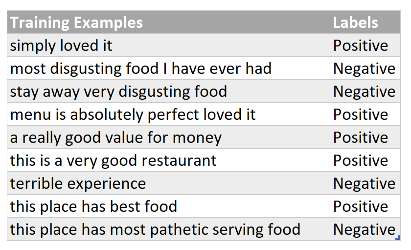
Preprocessed Training Dataset
Step #2 : Training Your Naïve Bayes Model
Just simply make two bag of words (BoW), one for each category, and each of them will simply contain words and their corresponding counts. All words belonging to “Positive” sentiment/label will go to one BoW and all words belonging to “Negative” sentiment will have their own BoW. Every sentence in training set is split into words (on the basis of space as a tokenizer/separator) and this is how simply word-count pairs are constructed as demonstrated below :
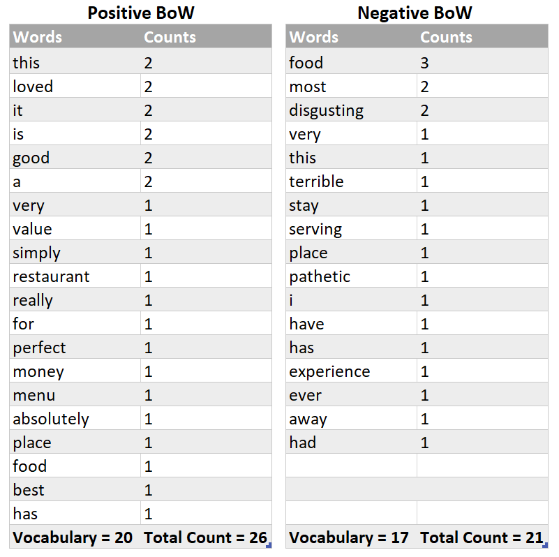
BoW for Both categories
We are done with the training of The Naive Bayes Model!
Milestone # 2 Achieved 👍
Grrreat! You have achieved two milestones ! 😃 👍 👍
Now its break time ! You can grab a cup of coffee or stretch your muscles before diving into the Grand Grand Grand Milestone # 3

Caution : We are about to begin the most essential part of the Naive Bayes Model i.e using the above trained model for prediction of restaurant reviews. I now It’s a bit lengthy but totally worth it as we will be discussing each and every minute detail leaving zero ambiguities as the end result !
The Grand Grand Grand Milestone # 3 Begins!
The Testing Phase — Where Prediction Comes into the Play!
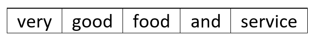
Consider that now your model is given a restaurant review, “Very good food and service!!!” , and it needs to classify to what particular category it belongs to. A positive review or a negative one? We need to find the probability of this given review of belonging to each category and then we would assign it either a positive or a negative label depending upon for which particular category this test example was able to score more probability.
Finding Probability of a Given Test Example
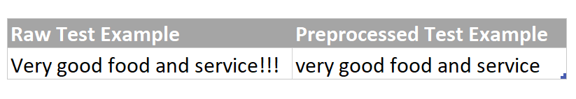
Step # 1 : Preprocessing of Test Example
Preprocess the test example in the same way as the training examples were preprocessed i.e changing examples to lower case and excluding everything apart from letters/alphabets.
Step # 2 : Tokenization of Preprocessed Test Example
Tokenize the test example i.e split it into single words.
A Quick Side Note : You must be already familiar with the term “ feature” in machine learning. Here, in Naive Bayes, each word in the vocabulary of each class of the training data set constitutes a categorical feature . This implies that counts of all the unique words (i.e vocabulary/vocab) of each class are basically a set of features for that particular class. And why do we need “counts” ? because we need a numeric representation of the categorical word features as the Naive Bayes Model/Algorithm requires numeric features to find out the probabilistic scores!
Step # 3 : Using Probability to Predict Label for Tokenized Test Example
The not so intimidating mathematical form of finding probability
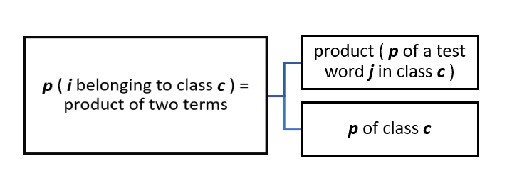
Probability of a Given Test Example i of belonging to class c
- let i = test example = “Very good food and service!!!”
- Total number of words in i = 5, so values of j ( representing feature number ) vary from 1 to 5. It’s that simple!
Let’s map the above scenario to the given test example to make it more clear!
Let’s start calculating values for these product terms
Step # 1 : Finding Value of the Term : p of class c
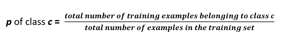
Simply the Fraction of Each Category/Class in the Training Set
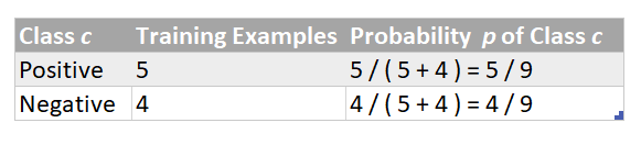
p of class c for Positive & Negative categories
Step # 2 : Finding value of term : product (p of a test word j in class c)
Before we start deducing probability of a test word j in a specific class c let’s quickly get familiar with some easy peasy notation that is being used in the not so distant lines of this blog post:
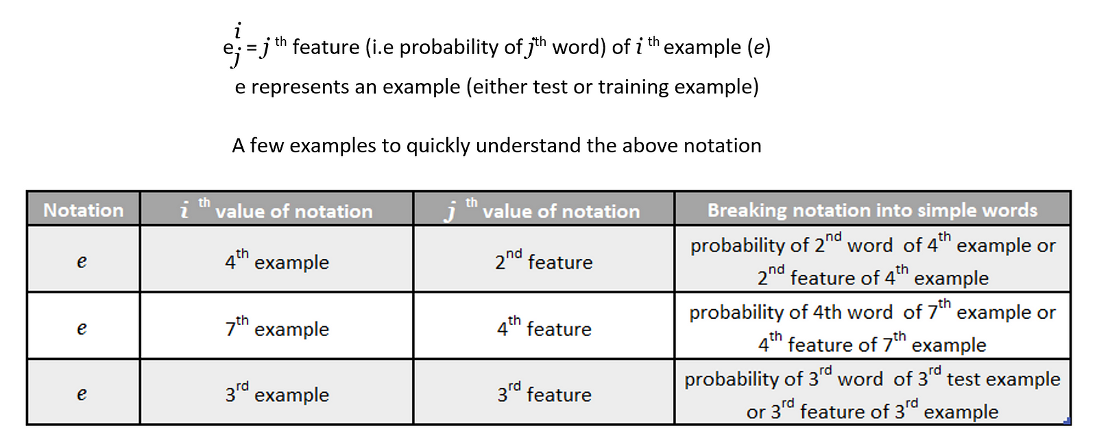
As we have only one example in our test set at the moment (for the sake of understanding), so i = 1.
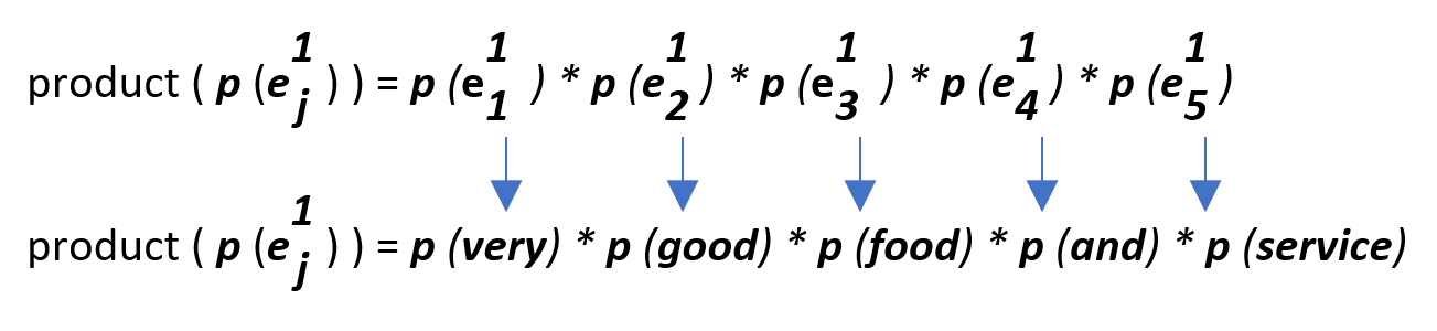
A Quick Side Note : During test time/prediction time, we map every word of test example against it’s count that was found during training phase . So, in this case, we are looking for in total 5 word counts for this given test example.

Just a random cat to keep you from falling asleep !
Finding Probability of a Test Word “ j ” in class c
Before we start calculating product ( p of a test word “ j ” in class c ), we obviously first need to determine p of a test word “ j ” in class c . There are two ways of doing this as specified below — which one should be actually followed and rather is practically used will be discovered in just a few minutes…
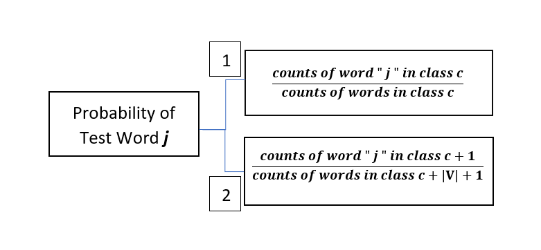
let’s first try finding probabilities using method number 1 :
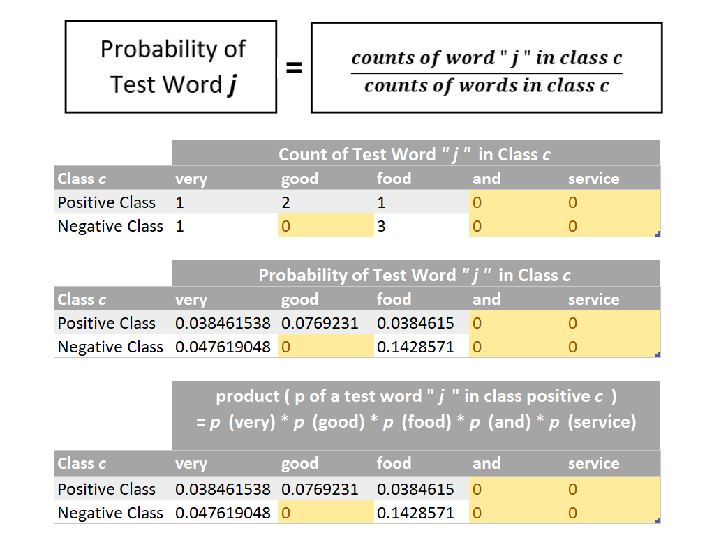
Now we can multiply the probabilities of individual words ( as found above ) in order to find the numerical value of the term :
product ( p of a test word “ j ” in class c )
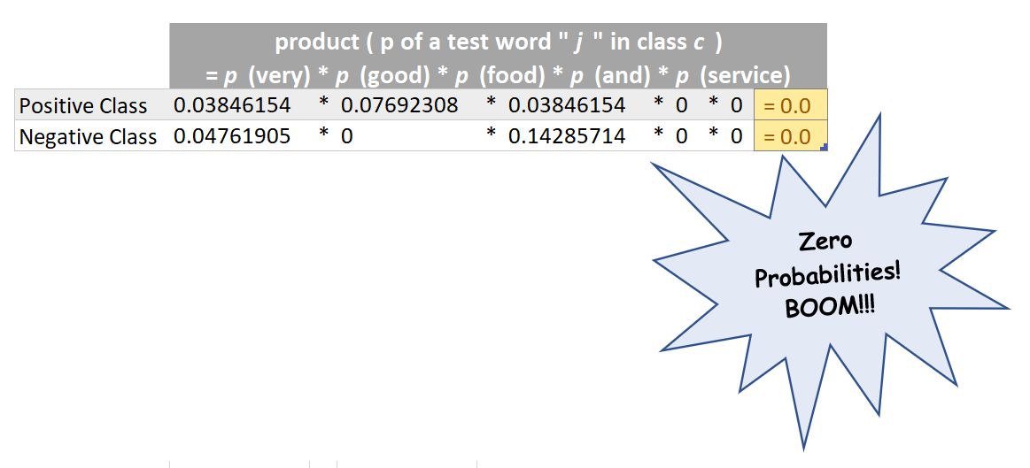
The Common Pitfall of Zero Probabilities!
By now, we have numerical values for both the terms i.e ( p of class c and product ( p of a test word “ j ” in class c ) ) for both the classes . So we can multiply both of these terms in order to determine p ( i belonging to class c ) for both the categories. This is demonstrated below :
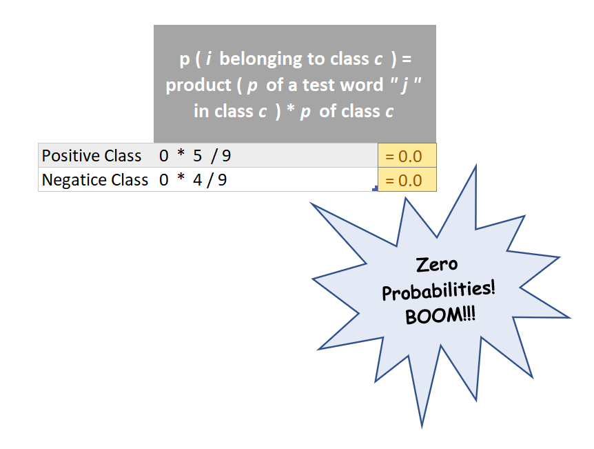
The Common Pitfall of Zero Probabilities!
The p ( i belonging to class c ) turns out to be zero for both the categories!!! but clearly the test example “Very good food and service!!!” belongs to positive class! Clearly, this happened because the product ( p of a test word
“ j ” in class c ) was zero for both the categories and this in turn was zero because a few words in the given test example (highlighted in orange) NEVER EVER appeared in our training dataset and hence their probability was zero! and clearly they have caused all the destruction!
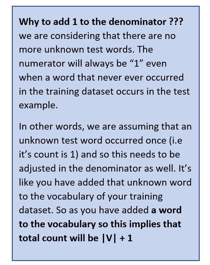
So does this imply that whenever a word that appears in the test example but never ever occurred in the training dataset will always cause such destruction ? and in such case our trained model will never be able to predict the correct sentiment? It will just randomly pick positive or negative category since both have same zero probability and predict wrongly? The answer is NO! This is where the second method (numbered 2) comes into play and infact this is the mathematical formula that is actually used to deduce p ( i belonging to class c ) . But before we move on the method number 2, we should first get familiar with it’s mathematical brainy stuff!
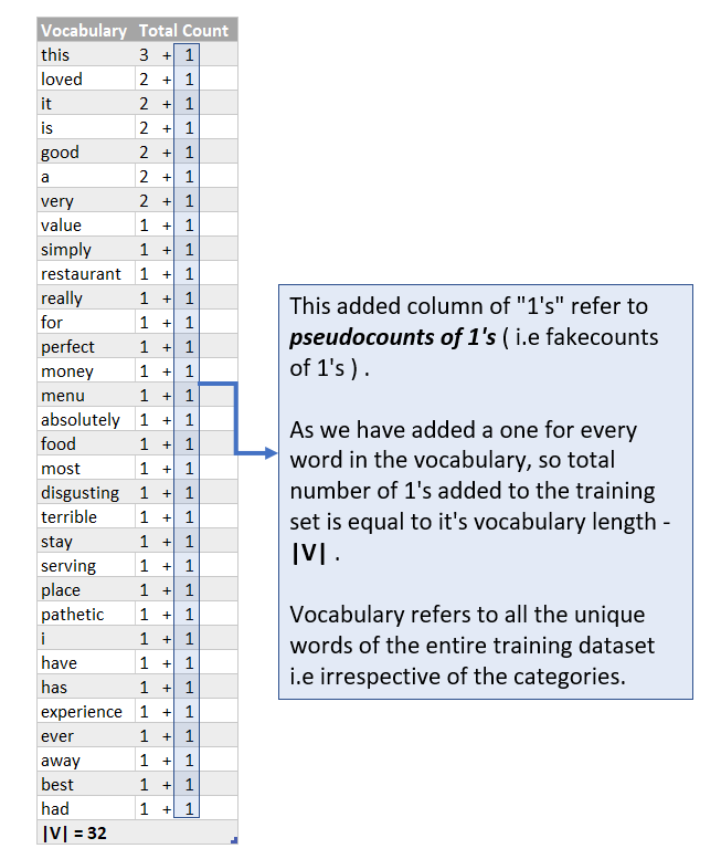
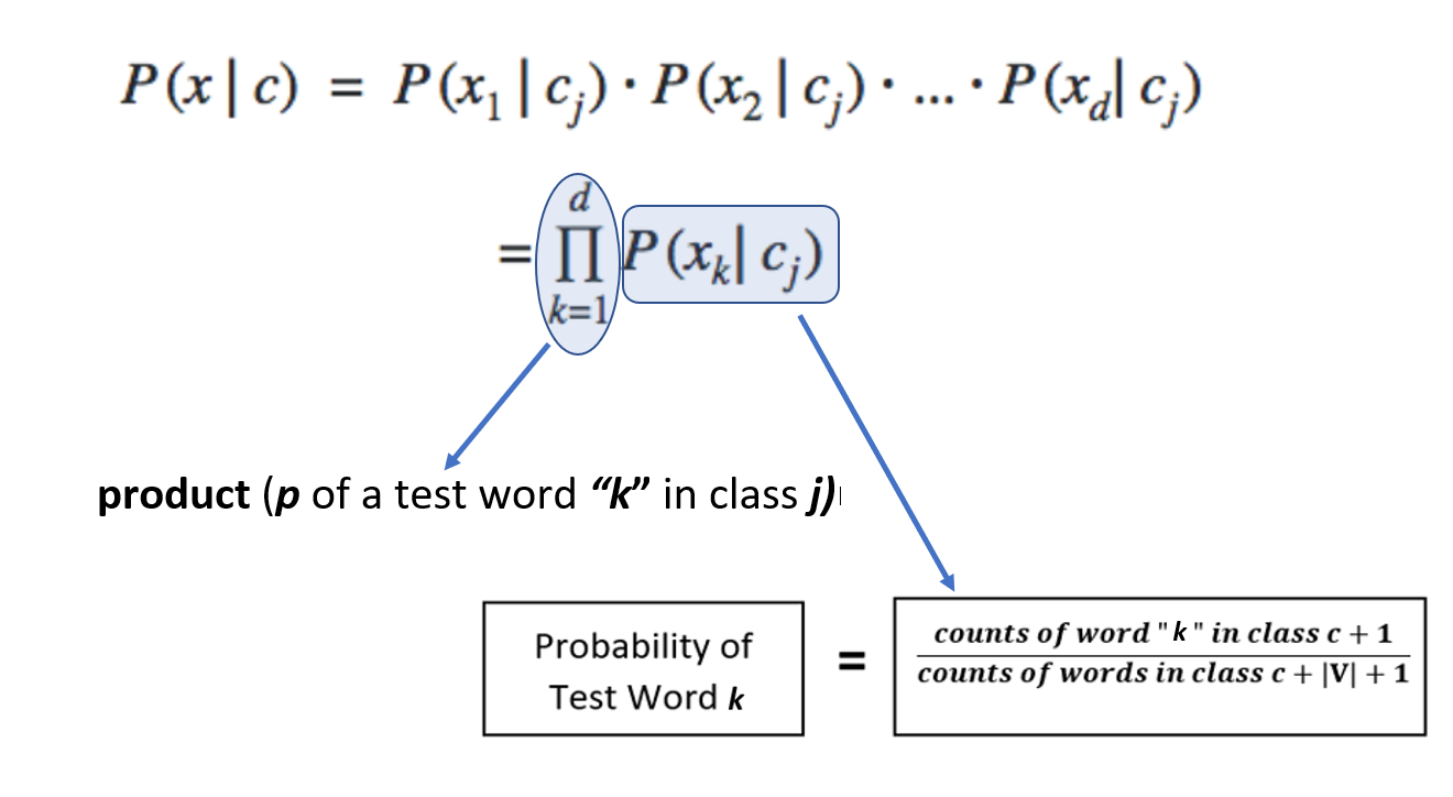
So now after adding pseudocounts of 1’s , the probability p of a test word that NEVER EVER APPEARED IN THE TRAINING DATASET WILL NEVER BE ZERO and therefore , the numerical value of the term product ( p of a test word “ j ” in class c ) will never end up as zero which in turn implies that
p ( i belonging to class c ) will never be zero as well! So all is well and no more destruction by zero probabilities!
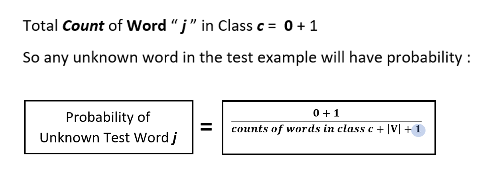
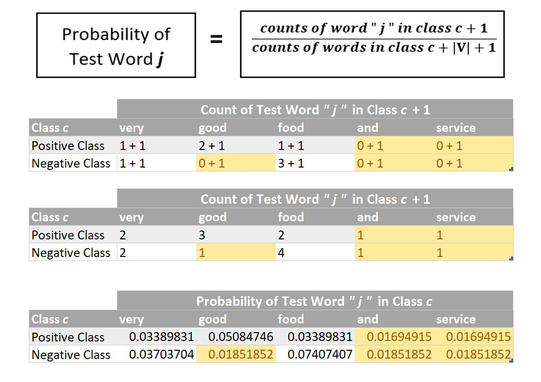
So the numerator term of method number 2 will have an added 1 as we have added a one for every word in the vocabulary and so it becomes :

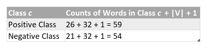
Similarly the denominator becomes :

And so the complete formula :
Probabilities of Positive & Negative Class
Yessssss ! You are almost there !
Now finding probabilities using method number 2 :
Handling of Zero Probabilities : These act like failsafe probabilities !
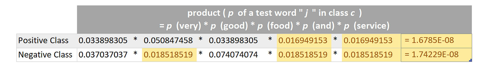
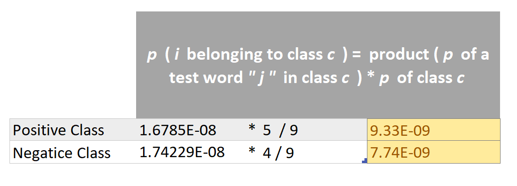
Now as probability of the test example, ”Very good food and service!!!” is more for the positive class i.e 9.33E-09 as compared to the negative class (i.e 7.74E-09), so we can predict it as a Positive Sentiment ! And that is how we simply predict a label for a test/unseen example
The Grand Grand Grand Milestone # 3 Achieved !! 👍 👍 👍
Only a few final touch-ups are remaining ! You can take a short break before we move towards the ending notes.
A Quick Side Note : As like every other machine learning algorithm, Naive Bayes too needs a validation set to assess the trained model’s effectiveness. But , since this post was aimed to focus on the algorithmic insights, so I deliberately avoided it and directly jumped to the testing part
Digging Deeper into the Mathematics of Probability
Now that you have built a basic understanding of the probabilistic calculations needed to train the Naive Bayes Model and then using it to predict probability for the given test sentence, I will now dig deeper into the probabilistic details.
While doing the calculations of probability of the given test sentence in the above section, we did nothing but implemented the given probabilistic formula for our prediction at test time:
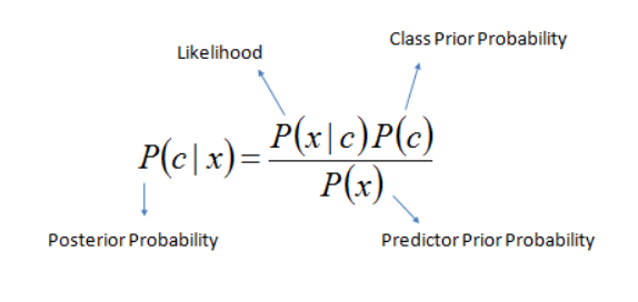
Decoding the above mathematical equation :
“ | ” = refers to a state which has already been given / or some filtering criteria
“ c ” = class/category
“ x ” = test example/test sentence
p (c|x) = given test example x , what is it’s probability of belonging to class c. This is also known as posterior probability. This is conditional probability that is to be found for the given test example x for each of the given training classes.
p(x|c)= given class c , what is the probability of example x belonging to class c. This is also known as likelihood as it implies how much likely does example x belongs to class c. This is conditional probability too as we are finding probability of x out of total instances of class c only i.e we have restricted/conditioned our search space to class c while finding the probability of x. We calculate this probability using the counts of words that are determined during the training phase.
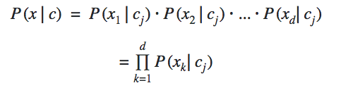
Here “ j ” represents a class and k represents a feature
We implicitly used this formula twice above in the calculations sections as we had two classes. Remember finding the numerical value of product ( p of a test word “ j ” in class c ) ?
p = This implies the probability of class c. This is also known as prior probability/unconditional probability. This is unconditional probability. We calculated this too earlier above in the probability calculations sections ( in Step # 1 which was finding value of term : p of class c )
p(x) = This is also known as normalizing constant so that the probability p(c|x) does actually falls in the range [0,1]. So if you remove this, the probability p(c|x) may not necessarily fall in the range of [0,1]. Intuitively this means probability of example x under any circumstances or irrespective of it’s class labels i.e whether positive or negative.
This is also reflected in total probability theorem which is used to calculate p(x) and dictates that to find p(x), we will find it’s probability in all given classes (because it is unconditional probability)and simply add them :
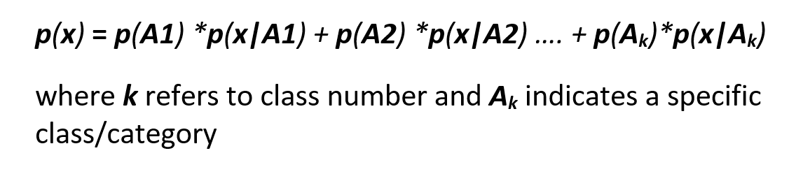
Total Probability Theorem
This implies that if we have two classes then we would have two terms, so in our particular case of positive and negative sentiments:
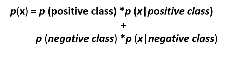
Total Probability Theorem for Two Classes
Did we use it in the above calculations? No we did not. Why??? because we are comparing probabilities of positive and negative class and since the denominator remains the same, so in this particular case, omitting out the same denominator doesn’t affect the prediction by our trained model. It simply cancels out for both classes. So although we can include it but there is no such logical reason to do so. But again as we have eliminated the normalization constant, the probability p(c|x) may not necessarily fall in the range of [0,1]
Milestone # 4 Achieved 👍
Avoiding the Common Pitfall of The Underflow Error!
- If you noticed, the numerical values of probabilities of words ( i.e p of a test word “ j ” in class c ) were quite small. And therefore, multiplying all these tiny probabilities to find product ( p of a test word “ j ” in class c ) will yield even a more smaller numerical value that often results in underflow which obviously means that for that given test sentence, the trained model will fail to predict it’s category/sentiment. So to avoid this underflow error, we take help of mathematical log as follows :
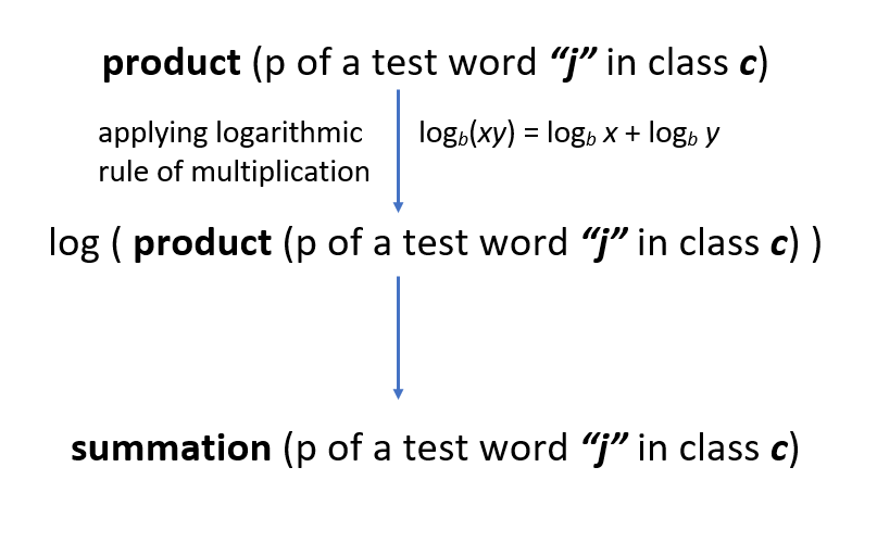
Avoiding the Underflow Error
- So now instead of multiplication of the tiny individual word probabilities, we will simply add them. And why only log? why not any other function? Because log increases or decreases monotonically which means that it will not affect the order of probabilities. Probabilities that were smaller will still stay smaller after the log has been applied on them and vice versa. so let’s say that a test word “is” has a smaller probability than the test word “happy”, so after passing these through log would although increase their magnitude but “is” would still have a smaller probability than “happy”. Therefore, without affecting the predictions of our trained model, we can effectively avoid the common pitfall of underflow error.
Milestone # 5 Achieved 👍
Concluding Notes….
- Although we live in a age of API’s and practically rarely code from scratch. But understanding the algorithmic theory in depth is extremely vital to develop a sound understanding of how the machine learning algorithms actually work. It is only the key understanding which actually differentiates a true data scientist from a na_i_ve one and what actually matters when training a really good model. So before moving to API’s , I personally believe that a true data scientist should code from scratch to actually see behind the numbers and the reason why a particular algorithm is better than the other.
- One of the best characteristics of the Na_ive Bayes_ Model is that you can improve it’s accuracy by simply updating it with new vocabulary words instead of always retraining it. You will just need to add words to the vocabulary and update the words counts accordingly. That’s it!

Photo Credits : Benjamin Davies on Unsplash
At last! Finally! Milestone # 6 Achieved 😤 😤 😤
So that’s all for this blog post aaaand you have taken a step forward in you ML journey — cheers! 😄
Upcoming posts will include :
- Unfolding Naïve Bayes from Scratch! Take-2 🎬 Implementation of Naive Bayes from Scratch in Python
- Unfolding Naïve Bayes from Scratch! Take-3 🎬 Implementation of Naive Bayes using scikit-learn (Python’s Holy grail of Machine Learning!)
Stay Tuned ! 📻
If you have any thoughts, comments, or questions, feel free to comment below or connect 📞 with me on aisha@TDS.com
If you liked my article, please clap 👏 as many times as you have enjoyed reading it (it fuels me to write more in-depth Data Science blogs 😃) and feel free to share it with your friends!
